Inverted pendulum aaaaaaaaaaaaaaaaaaaaaaaaaaaaaa
Bạn đang xem bản rút gọn của tài liệu. Xem và tải ngay bản đầy đủ của tài liệu tại đây (1.16 MB, 73 trang )
Inverted
Pendulum
Analysis, Design and
Implementation
IIEE Visionaries
Document Version 1.0
Reference:
The work included in this document has been carried out in the Instrumentation
and Control Lab at the Institute of Industrial Electronics Engineering, Karachi,
Pakistan.
CONTENTS
4
W HAT'S INSIDE T HIS REPORT
(CONTENTS IN DETAIL)
4
CONTENTS IN DETAIL
…
3
THE AUTHORS
…
6
PREFACE
…
9
INTRODUCTION
…
12
…
19
…
26
…
34
…
36
ü
ü
ABOUT THE AUTHOR
TECHNICAL ADVISOR
ü
ü
INTRODUCTION TO INVERTED PENDULUM
APPLICATIONS OF INVERTED PENDULUM
o SIMULATION OF DYNAMICS OF A ROCKET VEHICLE
o MODEL OF A HUMAN STANDING STILL
ü PROBLEM DESCRIPTION
MATHEMATICAL WORK
ü
MATHEMATICAL ANALYSIS
o SETUP DESCRIPTION
o INVERTED PENDULUM SYSTEM EQUATIONS
o ACTUATION MECHANISM
o TRANSFER FUNCTION OF THE W HOLE SYSTEM
ü SYSTEM P ARAMETERS
ANALYSIS OF UNCOMPENSATED SYSTEM
ü
ü
ü
ü
ü
ü
POLE ZERO MAP OF UNCOMPENSATED OPEN LOOP S YSTEM
IMPULSE RESPONSE OF UNCOMPENSATED OPEN LOOP S YSTEM
ROOT LOCUS OF THE UNCOMPENSATED S YSTEM
STEP RESPONSE OF UNCOMPENSATED OPEN LOOP S YSTEM
SIMULINK M ODEL FOR THE OPEN LOOP IMPULSE RESPONSE
SIMULINK M ODEL FOR THE OPEN LOOP STEP RESPONSE
COMPENSATION DESIGN
ü HOW CAN THE COMPENSATION BE DESIGNED?
(POSSIBLE OPTIONS)
ROOT LOCUS SYSTEM DESIGN
ü W HY COMPENSATION IS REQUIRED?
ü COMPENSATION GOALS
ü COMPENSATION DESIGN
T HE SISO DESIGN T OOL
ü W HAT IS THE SISO DESIGN TOOL
ü IMPORTING MODELS INTO THE SISO DESIGN TOOL
ü OPENING THE SISO DESIGN TOOL
ü DESIGN SPECIFICATIONS
ü ROOT LOCUS DESIGN WITH SISO DESIGN TOOL
ü ADDING POLES AND ZEROS TO THE COMPENSATOR
ü PROCEDURE
ANALYSIS OF COMPENSATED SYSTEM
…
43
…
56
…
61
CONCLUSION
…
63
APPENDIX
…
65
ü
ü
ü
ü
ü
ü
ü
POLE-ZERO MAP OF COMPENSATED OPEN LOOP S YSTEM
ROOT LOCUS OF THE COMPENSATED S YSTEM
POLE-ZERO MAP OF COMPENSATED CLOSED-LOOP S YSTEM
IMPULSE RESPONSE OF PID COMPENSATED SYSTEM
STEP RESPONSE OF PID COMPENSATED S YSTEM
CONCLUSION OF COMPENSATION ANALYSIS
SIMULINK M ODEL FOR CLOSED-LOOP STEP RESPONSE OF COMPENSATED
SYSTEM
ü SIMULINK M ODEL FOR CLOSED-LOOP IMPULSE RESPONSE OF COMPENSATED
SYSTEM
ü SIMULINK M ODEL FOR RESPONSE TO DISTURBANCE IN THE FORCE ON THE
CART OF COMPENSATED S YSTEM
ü SIMULINK M ODEL FOR RESPONSE TO DISTURBANCE IN THE POSITION OF
INVERTED BROOM OF COMPENSATED S YSTEM
PRACTICAL IMPLEMENTATION
ü CONTROLLER IMPLEMENTATION
ANALOG PID CONTROLLER DESIGNS
ü DESIGN 1: IDEAL PID ALGORITHM
ü DESIGN 2: P ARALLEL PID ALGORITHM
ü DESIGN 3: SERIES PID ALGORITHM
PRACTICAL RESULTS
ü EXPERIMENTAL DATA
ü M-FILE FOR D ATA OF THE INVENTED PENDULUM SYSTEM
ü M-FILE FOR OPEN LOOP & CLOSED LOOP (UNCOMPENSATED) TRANSFER
FUNCTION OF IP S YSTEM
ü M-FILE FOR ANALYSIS OF THE UNCOMPENSATED INVERTED PENDULUM S YSTEM
ü M-FILE FOR CLOSED LOOP COMPENSATED TRANSFER FUNCTION OF IP S YSTEM
ü M-FILE FOR ANALYSIS OF THE COMPENSATED INVERTED PENDULUM SYSTEM
ü M-FILE FOR PLOT OF E XPERIMENTAL DATA OBTAINED THRU 8051-B ASED DAQ CARD
BIBLIOGRAPHY
ü BOOKS
ü PAPERS
ü W EB
…
72
AUTHORS
œ
ABOUT THE AUTHOR
The “INVERTED PENDULUM, ANALYSIS, DESIGN AND
IMPLEMENTATION ” is a collection of MATLAB
functions and scripts, and SIMULINK models,
useful for analyzing Inverted Pendulum System and
designing Control System for it.
This collection is developed by:
K HALIL SULTAN
Khalil Sultan is currently pursuing the B.E. degree
in Industrial Electronics at the Institute of Industrial
Electronics Engineering (IIEE), PCSIR, NEDUET,
Karachi, Pakistan. He is a STUDENT MEMBER of the
IEEE, Inc. and INSTITUTION OF ENGINEERS,
PAKISTAN IEP.
He is the author of another Simulink Blockset
“SERVO SYSTEM BLOCKSET” which can also be
looked at MATLAB CENTRAL FILE E XCHANGE at
/>nge/loadFile.do?objectId=3087&objectType=FILE
He is also the author of another Simulink Block
“SINGLE PULSE GENERATOR ” which can also be
looked at MATLAB CENTRAL FILE E XCHANGE at
/>nge/loadFile.do?objectId=1762&objectType=FILE
The author can be approached at:
E-MAIL :
M AILING ADDRESS :
Khalil Sultan,
C/o Institute of Industrial Electronics Engineering
(IIEE), PCSIR.
ST-22/C, Block 6, Gulshan-e-Iqbal,
Karachi - 75300, Pakistan.
VOICE:
+ 92 - 21 - 6672896
FAX :
+ 92 - 21 - 4966274
TECHNICAL ADVISOR
ASHAB MIRZA, ASST. PROF.
Mr. Ashab Mirza is Assistant Professor at the
Institute of Industrial Electronics Engineering (IIEE),
PCSIR, Karachi, Pakistan. He received his B.E.
degree in Electronics from DCET, NEDUET,
Karachi, Pakistan in 1983 and the M.S. degree in
Aerospace Engineering from ENSAE (Sup’Aero),
Toulouse, France in 1987. He is currently pursuing
the Ph.D. degree at Pakistan Navy Engineering
College (PNEC), NUST, Karachi, Pakistan.
He joined INSTITUTE OF INDUSTRIAL ELECTRONICS
ENGINEERING (IIEE), Karachi in 1997 and is now an
assistant professor.
He is technical referee of AMSE (Association for
the Advancement of Modeling & Simulation
Techniques in Enterprises), for assessment of
technical papers for Control System journals. He is
also the technical reviewer of World Congress of
IFAC, held in 2002 at Barcelona, Spain. He is
technical reviewer of papers for the Conferences &
Seminars of IEEE Karachi Section and has helped
organize many international and national
conferences.
His research interest is control system design for
non linear and time-variant systems. He is working
in this area since 1988, after securing his MS
degree.
He is a SENIOR MEMBER of the IEEE.
He can be approached at:
E-MAIL :
M AILING ADDRESS :
Asst. Prof. Ashab Mirza,
C/o Institute of Industrial Electronics Engineering
(IIEE), PCSIR.
ST-22/C, Block 6, Gulshan-e-Iqbal,
Karachi - 75300, Pakistan.
VOICE:
+ 92 - 21 - 4982353
FAX :
+ 92 - 21 - 4966274
PREFACE
œ
PREFACE
œ
The “INVERTED PENDULUM, ANALYSIS, DESIGN AND IMPLEMENTATION ” is a collection of
MATLAB functions and scripts, and SIMULINK models, useful for analyzing Inverted
Pendulum System and designing Control System for it.
This report & MATLAB-files collection are developed as a part of practical assignment on
Control System Analysis, Design & Development practical problem. The assigned
problem of INVERTED PENDULUM is a part of Lab Work of Control System – III Course at
the INSTITUTE OF INDUSTRIAL ELECTRONICS ENGINEERING (IIEE), KARACHI, P AKISTAN .
The Inverted Pendulum is one of the most important classical problems of Control
Engineering. Broom Balancing (Inverted Pendulum on a cart) is a well known example
of nonlinear, unstable control problem. This problem becomes further complicated when
a flexible broom, in place of a rigid broom, is employed. Degree of complexity and
difficulty in its control increases with its flexibility. This problem has been a research
interest of control engineers.
Control of Inverted Pendulum is a Control Engineering project based on the FLIGHT
SIMULATION OF ROCKET OR MISSILE DURING THE INITIAL STAGES OF FLIGHT. The AIM OF THIS
STUDY is to stabilize the Inverted Pendulum such that the position of the carriage on the
track is controlled quickly and accurately so that the pendulum is always erected in its
inverted position during such movements.
This practical exercise is a presentation of the analysis and practical implementation of
the results of the solutions presented in the papers, “Robust Controller for Nonlinear
& Unstable System: Inverted Pendulum” [3] and “Flexible Broom Balancing” [4], in
which this complex problem was analyzed and a simple yet effective solution was
presented. The details of these papers can be looked in the BIBLIOGRAPHY section.
CONTENT OVERVIEW
This report comprises of EIGHT (8) major sections.
ü Section 1 introduces the classical control problem of Inverted Pendulum, and
provides the details of the problem from the control engineering aspects. It also
puts light on the possible applications of this problem.
ü Section 2 explores the mathematical model of the Inverted Pendulum System.
ü Section 3 provides the details of the analysis of the uncompensated system. The
analysis includes the pole-zero map, impulse response and step response of the
uncompensated open-loop system and root locus of the uncompensated system.
ü Section 4 explores the possible ways of designing the required control system
for the Inverted Pendulum System.
ü Section 5 explains how the control system can be designed using Root-Locus
techniques. The designing is done in MATLAB, using the SISO Design Tool. A
brief primer to SISO Design Tool is also included in the report in this section.
ü Section 6 provides the details of the analysis of the compensated system. The
analysis includes the pole-zero map of the PID compensated open-loop system
and root locus, impulse response and step response of the PID compensated
closed-loop system. In the conclusion of the Compensation Analysis section, it
has been overviewed that how much of the compensation goals have been
achieved.
ü Section 7 details the different ways of practically implementing the designed PID
controller. It shows different circuit configurations for achieving the required
transfer function.
ü Section 8 includes the practical results obtained recorded using a 8051-based
Data Acquisition Card. Then the obtained experimental data is filtered to remove
the unwanted high frequency components introduced due to sampling.
ü Appendix contains the MATLAB m-files, used for analyzing uncompensated
Inverted Pendulum System, designing Control System for it, and then analyzing
the PID compensated system.
ACKNOWLEDGEMENTS
We would like to thank the following reviewers for their useful suggestions, constructive
criticisms and helpful comments.
DR. KEN DUTTON
School of Engineering, Sheffield Hallam University, UK
Author: “Art of Control Engineering"
KHALIL SULTAN
July 25, 2003
SECTION 1
INTRODUCTION
œ
INTRODUCTION
i
Remember when you were a child and you tried to balance a broom-stick on your index
finger or the palm of your hand? You had to constantly adjust the position of your hand
to keep the object upright. An INVERTED PENDULUM does basically the same thing.
However, it is limited in that it only moves in one dimension, while your hand could move
up, down, sideways, etc.
Just like the broom-stick, an Inverted Pendulum is an inherently unstable system. Force
must be properly applied to keep the system intact. To achieve this, proper control
theory is required. The Inverted Pendulum is essential in the evaluating and comparing
of various control theories.
The inverted pendulum (IP) is among the most difficult systems to control in the field of
control engineering. Due to its importance in the field of control engineering, it has been
a task of choice to be assigned to Control Engineering students to analyze its model and
propose a linear compensator according to the PID control law. Being an unstable
system, Inverted Pendulum is very common control problem being assigned to a student
of Control System Engineering (from Bachelor to Postgraduate level), to control it's
dynamics.
The reasons for selecting the IP as the system are:
•
•
•
It is the most easily available system (in most academia) for laboratory usage.
It is a nonlinear system, which can be treated to be linear, without much error, for
quite a wide range of variation.
Provides a good practice for prospective control engineers.
The various stages of the work for accomplishing the task of controlling the Inverted
Pendulum are as follows:
•
•
•
•
•
Modeling the IP and linearizing the model for the operating range.
Analyzing the uncompensated closed loop response with the help of a root locus
plot.
Designing the PID controller and simulating it in MATLAB for proper tuning and
verification.
Analyzing the compensated closed loop response of the system.
Implementing the controller on the physical IP model.
APPLICATIONS OF INVERTED PENDULUM
i
Among the some considerable applications of inverted pendulum (IP) are:
ü SIMULATION OF DYNAMICS OF A ROBOTIC ARM
The Inverted Pendulum problem resembles the control systems that exist in robotic
arms. The dynamics of Inverted Pendulum simulates the dynamics of robotic arm in the
condition when the center of pressure lies below the centre of gravity for the arm so that
the system is also unstable. Robotic arm behaves very much like Inverted Pendulum
under this condition.
ü MODEL OF A HUMAN STANDING STILL
The ability to maintain stability while standing straight is of great importance for the daily
activities of people. The central nervous system (CNS) registers the pose and changes
in the pose of the human body, and activates muscles in order to maintain balance.
The inverted pendulum is widely accepted as an adequate model of a human standing
still (quiet standing).
An inverted pendulum (assuming no attached springs) is unstable, and it is hence
obvious that feedback of the state of the pendulum is needed to stabilize the pendulum.
Two models for the CNS feedback control are generally considered:
→ Time invariant, linear feedback control;
→ Linear feedback outside a threshold. No sensory feedback within the threshold.
There are certain passive mechanisms, such as stiffness in muscles and supportive
tissue, which may be modeled as a spring and damper.
INVERTED PENDULUM WITH
PASSIVE MECHANISMS MODELED
AS A SPRING AND DAMPER
The spring and damper leads to a negative feedback loop that could be enough to
stabilize the pendulum, if the spring is stiff enough.
More details about this application of Inverted Pendulum System can be looked at [15].
PROBLEM DEFINITION
Design a control system
that keeps the pendulum
balanced and tracks the
cart to a commanded
position!!!
It is virtually impossible to balance a pendulum in the inverted position without applying
some external force to the system. The Carriage Balanced Inverted Pendulum (CBIP)
system, shown below, allows this control force to be applied to the pendulum carriage.
This CBIP provides the control force to the carriage by means of a DC servo-motor
through a belt drive system. The outputs from the CBIP rig can be carriage position,
carriage velocity, pendulum angle and pendulum angular velocity (only pendulum angle
in our case). The pendulum angle is fed back to an Analog Controller which controls the
servo-motor, ensuring consistent and continuous traction. The AIM OF THE STUDY is to
stabilize the pendulum such that the position of the carriage on the track is controlled
quickly and accurately and that the pendulum is always maintained tightly in its inverted
position during such movements.
The problem involves a cart, able to move backwards and forwards, and a pendulum,
hinged to the cart at the bottom of its length such that the pendulum can move in the
same plane as the cart, shown below. That is, the pendulum mounted on the cart is free
to fall along the cart's axis of motion. The system is to be controlled so that the
pendulum remains balanced and upright, and is resistant to a step disturbance.
This problem involves A SIMPLE COUPLED SYSTEM. If the pendulum starts off-centre, it
will begin to fall. The pendulum is coupled to the cart, and the cart will start to move in
the opposite direction, just as moving the cart would cause the pendulum to become off
centre. As change to one of parts of the system results in change to the other part, this
is a more complicated control system than it appears at first glance. For this reason, this
problem is often used as a demonstration of fuzzy control.
The inverted pendulum cart runs along a track and is pulled by a belt connected to an
electric motor. A potentiometer measures the cart position from its rotation and another
potentiometer measures the angle of the pendulum.
If the output is the angle of the pendulum relative to the vertical axis (in upright position),
we realize that the system is unstable, since the pendulum will fall down if we release it
with a small angle. To stabilize the system, i.e., to keep the pendulum in upright position,
a feedback control system must be used.
Link 2
Link 1
The inverted pendulum is an excellent test bed for linear control theory. In this classic
inverted pendulum control experiment, we seek a feedback control law that balances
Link 2 in its unstable, inverted position. The first link undergoes linear translation, our
first link rotates.
The above photo shows the mechanism in its stable, pendant position.
So briefly, the Inverted Pendulum system is made up of a cart and a pendulum. The goal
of the controller is to move the cart to its commanded position without causing the
pendulum to tip over. In open loop this system is unstable.
THE TASK ASSIGNED IS: to analyze, design & develop a control loop for the given
inverted pendulum (with servomechanism).
Following is the over all block-diagram for the feedback control system: [NEXT P AGE]
U1
(DISTURBANCE IN
FORCE ON CART)
θR
e
A
_
PID
CONTROLLER
EF
U2
(DISTURBANCE IN
POSITION OF BROOM)
F
EA Cart Pulley
INVERTED
& ServoPENDULUM
mechanis
m SERVOMECHANISM
θC
POSITION FEEDBACK
Our implementation contains only feedback from the pendulum angle (that is, only one
out of the four states is used for feedback, the other states being carriage position,
carriage velocity and pendulum angular velocity). The implementation may be enhanced
by incorporation of cart-position control loop.
In this problem, the pendulum is first positioned upright manually, that is, in a position of
unstable equilibrium, or it is given some initial displacement (position). The controller is
then switched in to balance the pendulum and to maintain this balance in the presence
of disturbances. A simple disturbance may be a light tap on the balanced pendulum. A
complex disturbance may be gusts of wind (use a fan!).
This setup can be used to study the control of open loop unstable system. It is a
demonstration of the stabilizing benefits of feedback control. A range of control
techniques ranging from the simple phase advance compensator to neural net
controllers can be applied.
SECTION 2
MATHEMATICAL W ORK
MATHEMATICAL ANALYSIS
i
An inverted pendulum is a classic control problem. The process is non linear and
unstable with one input signal and several output signals. The aim is to balance a
pendulum vertically on a motor driven wagon.
The following figure shows an inverted pendulum. The aim is to move the wagon along
the x direction to a desired point without the pendulum falling. The wagon is driven by a
DC motor, which is controlled by a controller (analog in our implementation). The
wagons x position (not in our case) and the pendulum angle è are measured and
supplied to the control system. A disturbance force, FDISTURBANCE, can be applied on top
of the pendulum.
A mathematical model of the system has been developed, giving the angle of the
pendulum resulting from a force applied to the base.
Setup Description
The inverted pendulum is mounted on a moving cart. A servomotor is controlling the
translation motion of the cart, through a belt/pulley mechanism. That is, the cart is
coupled with a servo dc-motor through pulley and belt mechanism. The motor is derived
by servo electronics, which also contains controller-circuits. A rotary-potentiometer
is used to feedback the angular motion of the pendulum to servo electronics to generate
actuating-signal.
Controller circuits process the error signal, which then drives the cart through the
servomotor and driving pulley/belt mechanism. To-or/and-fro motion of the cart applies
moments on the inverted pendulum and thus it keeps the pendulum upright.
Inverted Pendulum System Equations
The Free Body Diagram of the system is used to obtain the equations of motion. Below
are the two Free Body Diagrams of the system.
Summing the forces in the Free Body Diagram of the cart in the horizontal direction, you
get the following equation of motion:
Mx&& + bx& + N = F
[1]
Note that you could also sum the forces in the vertical direction, but no useful
information would be gained. The sum of forces in the vertical direction is not considered
because there is no motion in this direction and we consider that the reaction force of the
earth balances all the vertical forces.
The force exerted in the horizontal direction due to the moment on the pendulum is
determined as follows:
τ = r × F = I θ&&
Iθ&&
F=
r
ml 2θ&&
=
l
= mlθ&&
&&
Component of this force in the direction of N is mlθcos
θ.
The component of the centripetal force acting along the horizontal axis is as follows:
I θ& 2
r
ml 2θ& 2
=
l
= mlθ& 2
F=
Component of this force in the direction of N is mlθ& 2 sinθ .
Summing the forces in the Free Body Diagram of the pendulum in the horizontal
direction, you can get an equation for N:
[2]
N = m &x& + mlθ&& cos θ − mlθ& 2 sinθ
If you substitute this equation [2] into the first equation [1], you get the first equation of
motion for this system:
[3]
(M + m ) &x& + bx& + mlθ&& cosθ − mlθ& 2 sinθ = F
To get the second equation of motion, sum the forces perpendicular to the pendulum.
This axis is chosen to simplify mathematical complexity. Solving the system along this
axis ends up saving you a lot of algebra. Just as the previous equation is obtained, the
vertical components of those forces are considered here to get the following equation:
[4]
P sinθ + N cosθ − mg sinθ = mlθ&& + m &x& cos θ
To get rid of the P and N terms in the equation above, sum the moments around the
centroid of the pendulum to get the following equation:
[5]
− Pl sinθ − Nl cos θ = Iθ&&
Combining these last two equations, you get the second dynamic equation:
[6]
(I + ml 2 )θ&& + mgl sinθ = −ml&x& cos θ
The set of equations completely defining the dynamics of the inverted pendulum are:
[3]
(M + m ) &x& + bx& + mlθ&& cosθ − mlθ& 2 sinθ = F
[6]
(I + ml 2 )θ&& + mgl sinθ = −ml&x& cos θ
These two equations are non-linear and need to be linearized for the operating range.
Since the pendulum is being stabilized at an unstable equilibrium position, which is ‘Pi’
radians from the stable equilibrium position, this set of equations should be linearized
about theta = Pi. Assume that theta = Pi + ø, (where ø represents a small angle from the
vertical upward direction).
Therefore, cos (theta) = -1, sin (theta) = -ø, and (d(theta)/dt)^2 = 0.
After linearization the two equations of motion become (where u represents the input):
[7]
(M + m ) &x& + bx& − mlφ&& = u
[8]
(I + ml 2 )φ&& − mglφ = mlx&&
To obtain the transfer function of the linearized system equations analytically, we must
first take the Laplace transform of the system equations. The Laplace transforms are:
(M + m ) X (s )s 2 + bX ( s )s − mlΦ( s )s 2 = U (s )
(I + ml 2 )Φ(s )s 2 − mglΦ(s ) = mlX ( s )s 2
When finding the transfer function, initial conditions are assumed to be zero. The
transfer function relates the variation from desired position [Output] to the force on the
cart [Input].
Since we will be looking at the angle Phi as the output of interest, solve the first equation
for X(s),
X (s ) = [
( I + ml 2 ) g
− 2 ]Φ (s )
ml
s
Then, substituting into the second equation will yield:
(M + m )[
(I + ml 2 ) g
(I + ml 2 ) g
+ ] Φ (s ).s2 + b[
+ ] Φ(s ).s − mlΦ (s ).s2 = U( s )
ml
s
ml
s
Re-arranging, the transfer function is:
ml 2
⋅s
Φ(s )
q
=
U( s )
b(I + ml 2 ) 3 mgl(M + m ) 2 bmgl
s4 +
⋅s −
⋅s −
.s
q
q
q
where,
q = (M + m )( I + ml 2 ) − ( ml ) 2 .
From the transfer function above it can be seen that there is both a pole and a zero at
the origin. These can be canceled and the transfer function becomes:
ml
⋅s
Φ(s )
q
=
U( s )
b(I + ml 2 ) 2 mgl(M + m )
bmgl
s3 +
⋅s −
⋅s −
q
q
q
The transfer function can thus be simplified as:
Φ(s )
ml ⋅ s
=
3
2
U( s ) q ⋅ s + b( I + ml ) ⋅ s 2 − mgl(M + m ) ⋅ s − bmgl
where q = ( M + m )(I + ml 2 ) − (ml ) 2 .
If we
then
NEGLECT THE FRICTION
in the system, that is, we take the coefficient of friction b=0,
Φ (s )
Kp
= 2
U ( s ) s Ap 2 − 1
where Kp =
1
( M + m )mgl
, and Ap = ±
(M + m )g
(M + m )(I + ml 2 ) − ( ml )2
Thus, the LINEARIZED APPROXIMATION TRANSFER FUNCTION for the IP has been obtained.
In time domain, the transfer function can be stated as:
Φ(t )
Kp
=
u( t ) D 2 / Ap2 - 1
Actuation Mechanism
The actuation mechanism consists of a movable cart (on rail), driven by a DC motor via
a pulley and belt. So the overall transfer function of the actuation mechanism will
depend upon the transfer function of “the DC Motor” and “the Pulley, Belt & Cart”.
P ULLEY, B ELT & CART
Load-Inertia to the motor consists of pulley (of radius r) and masses of cart and
pendulum. The load-torque, to be delivered by the motor is given as:
TL = (M + m).r 2 .D ω
TL ∝ r2 and F ∝ r
Note:
MOTOR
The dynamics of motor will also affect the transfer function of the actuation mechanism.
Experimental transfer function for the armature-controlled servo dc-motor is given as:
ω = Km
E
τD + 1
Where τ is the time constant, and it depends upon the load drive. That is, heavier the
load higher will be the value ofτ
τ . KM (radians/second/volts) is steady-state gain.
So the overall transfer function of the actuation mechanism is:
U( s )
( M + m )rs
= Km
E (s )
(τm s + 1)
Transfer Function of the Whole System
Open loop and linearized transfer function for the whole (uncontrolled) system can be
given as:
Φ(s )
=K
E( s )
where
s
(τm s + 1)(
s2
− 1)
Ap 2
K = KF KP KM r (M+m),
E (s) = Error Voltage, and
Φ (s) = Angular Position of the Pendulum.
Most of the modelling and system analysis has been taken from [3],[4] and [13].
SYSTEM PARAMETERS
The physical parameters of the system prototype are tabulated as follows:
M
m
b
L
I
R
τM
KM
KF
F
x
θ
Mass of the Cart
Mass of the Pendulum
Friction of the Cart
Length of pendulum to Center of Gravity
Moment of Inertia (Pendulum)
Radius of Pulley,
Time Constant of motor
Gain of Motor
Gain of Feedback
Force applied to the cart
Cart Position Coordinate
Pendulum Angle with the vertical
900 gm
100 gm
0.000 N/m/sec
23.5 cm
5.3 gm-m 2
2.3 cm
0.5 second
17 rad/sec/V
9/π V/rad/sec