Data Cleaning Using R
Bạn đang xem bản rút gọn của tài liệu. Xem và tải ngay bản đầy đủ của tài liệu tại đây (408.15 KB, 53 trang )
Discussion Paper
An introduction to data
cleaning with R
The views expressed in this paper are those of the author(s) and do not necesarily reflect
the policies of Statistics Netherlands
2013 | 13
Edwin de Jonge
Mark van der Loo
Publisher
Statistics Netherlands
Henri Faasdreef 312, 2492 JP The Hague
www.cbs.nl
Prepress: Statistics Netherlands, Grafimedia
Design: Edenspiekermann
Information
Telephone +31 88 570 70 70, fax +31 70 337 59 94
Via contact form: www.cbs.nl/information
Where to order
Fax +31 45 570 62 68
ISSN 1572-0314
© Statistics Netherlands, The Hague/Heerlen 2013.
Reproduction is permitted, provided Statistics Netherlands is quoted as the source.
60083 201313- X-10-13
An introduction to data cleaning
with R
Edwin de Jonge and Mark van der Loo
Summary. Data cleaning, or data preparation is an essential part of statistical analysis. In fact,
in practice it is often more time-consuming than the statistical analysis itself. These lecture
notes describe a range of techniques, implemented in the R statistical environment, that allow
the reader to build data cleaning scripts for data suffering from a wide range of errors and
inconsistencies, in textual format. These notes cover technical as well as subject-matter related
aspects of data cleaning. Technical aspects include data reading, type conversion and string
matching and manipulation. Subject-matter related aspects include topics like data checking,
error localization and an introduction to imputation methods in R. References to relevant
literature and R packages are provided throughout.
These lecture notes are based on a tutorial given by the authors at the useR!2013 conference in
Albacete, Spain.
Keywords: methodology, data editing, statistical software
An introduction to data cleaning with R
3
Contents
1
Notes to the reader . . . . . . . . . . . . . . . . . . . . . . . . . . . . . . . . . . . .
6
Introduction
7
1.1
Statistical analysis in five steps . . . . . . . . . . . . . . . . . . . . . . . . . . .
7
1.2
Some general background in R . . . . . . . . . . . . . . . . . . . . . . . . . . .
8
1.2.1
Variable types and indexing techniques . . . . . . . . . . . . . . . . . .
8
1.2.2
Special values . . . . . . . . . . . . . . . . . . . . . . . . . . . . . . . .
10
Exercises . . . . . . . . . . . . . . . . . . . . . . . . . . . . . . . . . . . . . . . . . .
11
2 From raw data to technically correct data
2.1
Technically correct data in R . . . . . . . . . . . . . . . . . . . . . . . . . . . . .
12
2.2
Reading text data into a R data.frame . . . . . . . . . . . . . . . . . . . . . . .
12
2.2.1
read.table and its cousins
. . . . . . . . . . . . . . . . . . . . . . . .
13
2.2.2
Reading data with readLines . . . . . . . . . . . . . . . . . . . . . . .
15
Type conversion . . . . . . . . . . . . . . . . . . . . . . . . . . . . . . . . . . .
18
2.3.1
Introduction to R's typing system . . . . . . . . . . . . . . . . . . . . . .
19
2.3.2
Recoding factors . . . . . . . . . . . . . . . . . . . . . . . . . . . . . .
20
2.3.3
Converting dates . . . . . . . . . . . . . . . . . . . . . . . . . . . . . .
20
character manipulation . . . . . . . . . . . . . . . . . . . . . . . . . . . . . .
23
2.4.1
String normalization . . . . . . . . . . . . . . . . . . . . . . . . . . . .
23
2.4.2
Approximate string matching . . . . . . . . . . . . . . . . . . . . . . .
24
Character encoding issues . . . . . . . . . . . . . . . . . . . . . . . . . . . . .
26
Exercises . . . . . . . . . . . . . . . . . . . . . . . . . . . . . . . . . . . . . . . . . .
29
From technically correct data to consistent data
31
3.1
Detection and localization of errors . . . . . . . . . . . . . . . . . . . . . . . . .
31
3.1.1
Missing values . . . . . . . . . . . . . . . . . . . . . . . . . . . . . . . .
31
3.1.2
Special values . . . . . . . . . . . . . . . . . . . . . . . . . . . . . . . .
33
3.1.3
Outliers . . . . . . . . . . . . . . . . . . . . . . . . . . . . . . . . . . .
33
3.1.4
Obvious inconsistencies . . . . . . . . . . . . . . . . . . . . . . . . . .
35
3.1.5
Error localization . . . . . . . . . . . . . . . . . . . . . . . . . . . . . .
37
Correction . . . . . . . . . . . . . . . . . . . . . . . . . . . . . . . . . . . . . .
39
3.2.1
Simple transformation rules . . . . . . . . . . . . . . . . . . . . . . . .
40
3.2.2
Deductive correction . . . . . . . . . . . . . . . . . . . . . . . . . . . .
42
3.2.3
Deterministic imputation . . . . . . . . . . . . . . . . . . . . . . . . . .
43
Imputation . . . . . . . . . . . . . . . . . . . . . . . . . . . . . . . . . . . . . .
45
3.3.1
Basic numeric imputation models . . . . . . . . . . . . . . . . . . . . .
45
3.3.2
Hot deck imputation . . . . . . . . . . . . . . . . . . . . . . . . . . . .
47
2.3
2.4
2.5
3
12
3.2
3.3
An introduction to data cleaning with R
4
3.3.3
kNN-imputation . . . . . . . . . . . . . . . . . . . . . . . . . . . . . .
48
3.3.4
Minimal value adjustment . . . . . . . . . . . . . . . . . . . . . . . . .
49
Exercises . . . . . . . . . . . . . . . . . . . . . . . . . . . . . . . . . . . . . . . . . .
51
An introduction to data cleaning with R 5
Notes to the reader
This tutorial is aimed at users who have some R programming experience. That is, the reader is
expected to be familiar with concepts such as variable assignment, vector, list, data.frame,
writing simple loops, and perhaps writing simple functions. More complicated constructs, when
used, will be explained in the text. We have adopted the following conventions in this text.
Code. All code examples in this tutorial can be executed, unless otherwise indicated. Code
examples are shown in gray boxes, like this:
1 + 1
## [1] 2
where output is preceded by a double hash sign ##. When code, function names or arguments
occur in the main text, these are typeset in fixed width font, just like the code in gray boxes.
When we refer to R data types, like vector or numeric these are denoted in fixed width font as
well.
Variables. In the main text, variables are written in slanted format while their values (when
textual) are written in fixed-width format. For example: the Marital status is unmarried.
Data. Sometimes small data files are used as an example. These files are printed in the
document in fixed-width format and can easily be copied from the pdf file. Here is an example:
1
2
3
4
5
%% Data on the Dalton Brothers
Gratt ,1861,1892
Bob ,1892
1871,Emmet ,1937
% Names, birth and death dates
Alternatively, the files can be found at />Tips. Occasionally we have tips, best practices, or other remarks that are relevant but not part
of the main text. These are shown in separate paragraphs as follows.
Tip. To become an R master, you must practice every day.
Filenames. As is usual in R, we use the forward slash (/) as file name separator. Under windows,
one may replace each forward slash with a double backslash \\.
References. For brevity, references are numbered, occurring as superscript in the main text.
An introduction to data cleaning with R
6
1 Introduction
Analysis of data is a process of inspecting, cleaning, transforming, and modeling
data with the goal of highlighting useful information, suggesting conclusions, and
supporting decision making.
Wikipedia, July 2013
Most statistical theory focuses on data modeling, prediction and statistical inference while it is
usually assumed that data are in the correct state for data analysis. In practice, a data analyst
spends much if not most of his time on preparing the data before doing any statistical operation.
It is very rare that the raw data one works with are in the correct format, are without errors, are
complete and have all the correct labels and codes that are needed for analysis. Data Cleaning is
the process of transforming raw data into consistent data that can be analyzed. It is aimed at
improving the content of statistical statements based on the data as well as their reliability.
Data cleaning may profoundly influence the statistical statements based on the data. Typical
actions like imputation or outlier handling obviously influence the results of a statistical
analyses. For this reason, data cleaning should be considered a statistical operation, to be
performed in a reproducible manner. The R statistical environment provides a good
environment for reproducible data cleaning since all cleaning actions can be scripted and
therefore reproduced.
1.1 Statistical analysis in ive steps
In this tutorial a statistical analysis is viewed as the result of a number of data processing steps
where each step increases the ``value'' of the data* .
data cleaning
Raw .data
type checking, normalizing
Technically
correct data
fix and impute
Consistent data
estimate, analyze, derive, etc.
Statistical results
tabulate, plot
Figure 1 shows an overview of a typical data
analysis project. Each rectangle represents
data in a certain state while each arrow
represents the activities needed to get from
one state to the other. The first state (Raw
data) is the data as it comes in. Raw data
files may lack headers, contain wrong data
types (e.g. numbers stored as strings), wrong
category labels, unknown or unexpected
character encoding and so on. In short,
reading such files into an R data.frame
directly is either difficult or impossible
without some sort of preprocessing.
Once this preprocessing has taken place,
data can be deemed Technically correct.
That is, in this state data can be read into
Figure 1: Statistical analysis value chain
an R data.frame, with correct names, types
and labels, without further trouble. However,
that does not mean that the values are error-free or complete. For example, an age variable
may be reported negative, an under-aged person may be registered to possess a driver's license,
or data may simply be missing. Such inconsistencies obviously depend on the subject matter
Formatted output
* In fact, such a value chain is an integral part of Statistics Netherlands business architecture.
An introduction to data cleaning with R
7
that the data pertains to, and they should be ironed out before valid statistical inference from
such data can be produced.
Consistent data is the stage where data is ready for statistical inference. It is the data that most
statistical theories use as a starting point. Ideally, such theories can still be applied without
taking previous data cleaning steps into account. In practice however, data cleaning methods
like imputation of missing values will influence statistical results and so must be accounted for in
the following analyses or interpretation thereof.
Once Statistical results have been produced they can be stored for reuse and finally, results can
be Formatted to include in statistical reports or publications.
Best practice. Store the input data for each stage (raw, technically correct,
consistent, aggregated and formatted) separately for reuse. Each step between the
stages may be performed by a separate R script for reproducibility.
Summarizing, a statistical analysis can be separated in five stages, from raw data to formatted
output, where the quality of the data improves in every step towards the final result. Data
cleaning encompasses two of the five stages in a statistical analysis, which again emphasizes its
importance in statistical practice.
1.2 Some general background in R
We assume that the reader has some proficiency in R. However, as a service to the reader, below
we summarize a few concepts which are fundamental to working with R, especially when
working with ``dirty data''.
1.2.1 Variable types and indexing techniques
If you had to choose to be proficient in just one R-skill, it should be indexing. By indexing we
mean all the methods and tricks in R that allow you to select and manipulate data using
logical, integer or named indices. Since indexing skills are important for data cleaning, we
quickly review vectors, data.frames and indexing techniques.
The most basic variable in R is a vector. An R vector is a sequence of values of the same type.
All basic operations in R act on vectors (think of the element-wise arithmetic, for example). The
basic types in R are as follows.
numeric
integer
factor
ordered
character
raw
Numeric data (approximations of the real numbers, ℝ)
Integer data (whole numbers, ℤ)
Categorical data (simple classifications, like gender)
Ordinal data (ordered classifications, like educational level)
Character data (strings)
Binary data
All basic operations in R work element-wise on vectors where the shortest argument is recycled
if necessary. This goes for arithmetic operations (addition, subtraction,…), comparison
operators (==, <=,…), logical operators (&, |, !,…) and basic math functions like sin, cos, exp
and so on. If you want to brush up your basic knowledge of vector and recycling properties, you
can execute the following code and think about why it works the way it does.
An introduction to data cleaning with R
8
# vectors have variables of _one_ type
c(1, 2, "three")
# shorter arguments are recycled
(1:3) * 2
(1:4) * c(1, 2)
# warning! (why?)
(1:4) * (1:3)
Each element of a vector can be given a name. This can be done by passing named arguments to
the c() function or later with the names function. Such names can be helpful giving meaning to
your variables. For example compare the vector
x <- c("red", "green", "blue")
with the one below.
capColor = c(huey = "red", duey = "blue", louie = "green")
Obviously the second version is much more suggestive of its meaning. The names of a vector
need not be unique, but in most applications you'll want unique names (if any).
Elements of a vector can be selected or replaced using the square bracket operator [ ]. The
square brackets accept either a vector of names, index numbers, or a logical. In the case of a
logical, the index is recycled if it is shorter than the indexed vector. In the case of numerical
indices, negative indices omit, in stead of select elements. Negative and positive indices are not
allowed in the same index vector. You can repeat a name or an index number, which results in
multiple instances of the same value. You may check the above by predicting and then verifying
the result of the following statements.
capColor["louie"]
names(capColor)[capColor == "blue"]
x <- c(4, 7, 6, 5, 2, 8)
I <- x < 6
J <- x > 7
x[I | J]
x[c(TRUE, FALSE)]
x[c(-1, -2)]
Replacing values in vectors can be done in the same way. For example, you may check that in
the following assignment
x <- 1:10
x[c(TRUE, FALSE)] <- 1
every other value of x is replaced with 1.
A list is a generalization of a vector in that it can contain objects of different types, including
other lists. There are two ways to index a list. The single bracket operator always returns a
sub-list of the indexed list. That is, the resulting type is again a list. The double bracket
operator ([[ ]]) may only result in a single item, and it returns the object in the list itself.
Besides indexing, the dollar operator $ can be used to retrieve a single element. To understand
the above, check the results of the following statements.
L <- list(x = c(1:5), y = c("a", "b", "c"), z = capColor)
L[[2]]
L$y
L[c(1, 3)]
L[c("x", "y")]
L[["z"]]
An introduction to data cleaning with R
9
Especially, use the class function to determine the type of the result of each statement.
A data.frame is not much more than a list of vectors, possibly of different types, but with
every vector (now columns) of the same length. Since data.frames are a type of list, indexing
them with a single index returns a sub-data.frame; that is, a data.frame with less columns.
Likewise, the dollar operator returns a vector, not a sub-data.frame. Rows can be indexed
using two indices in the bracket operator, separated by a comma. The first index indicates rows,
the second indicates columns. If one of the indices is left out, no selection is made (so
everything is returned). It is important to realize that the result of a two-index selection is
simplified by R as much as possible. Hence, selecting a single column using a two-index results
in a vector. This behaviour may be switched off using drop=FALSE as an extra parameter. Here
are some short examples demonstrating the above.
d <- data.frame(x = 1:10, y = letters[1:10], z = LETTERS[1:10])
d[1]
d[, 1]
d[, "x", drop = FALSE]
d[c("x", "z")]
d[d$x > 3, "y", drop = FALSE]
d[2, ]
1.2.2 Special values
Like most programming languages, R has a number of Special values that are exceptions to the
normal values of a type. These are NA, NULL, ±Inf and NaN. Below, we quickly illustrate the
meaning and differences between them.
NA Stands for not available. NA is a placeholder for a missing value. All basic operations in R
handle NA without crashing and mostly return NA as an answer whenever one of the input
arguments is NA. If you understand NA, you should be able to predict the result of the
following R statements.
NA + 1
sum(c(NA, 1, 2))
median(c(NA, 1, 2, 3), na.rm = TRUE)
length(c(NA, 2, 3, 4))
3 == NA
NA == NA
TRUE | NA
The function is.na can be used to detect NA's.
NULL You may think of NULL as the empty set from mathematics. NULL is special since it has no
class (its class is NULL) and has length 0 so it does not take up any space in a vector. In
particular, if you understand NULL, the result of the following statements should be clear to
you without starting R.
length(c(1, 2, NULL, 4))
sum(c(1, 2, NULL, 4))
x <- NULL
c(x, 2)
The function is.null can be used to detect NULL variables.
Inf Stands for infinity and only applies to vectors of class numeric. A vector of class integer can
never be Inf. This is because the Inf in R is directly derived from the international standard
for floating point arithmetic 1 . Technically, Inf is a valid numeric that results from
calculations like division of a number by zero. Since Inf is a numeric, operations between Inf
and a finite numeric are well-defined and comparison operators work as expected. If you
understand Inf, the result of the following statements should be clear to you.
An introduction to data cleaning with R
10
pi/0
2 * Inf
Inf - 1e+10
Inf + Inf
3 < -Inf
Inf == Inf
NaN Stands for not a number. This is generally the result of a calculation of which the result is
unknown, but it is surely not a number. In particular operations like 0/0, Inf-Inf and
Inf/Inf result in NaN. Technically, NaN is of class numeric, which may seem odd since it is
used to indicate that something is not numeric. Computations involving numbers and NaN
always result in NaN, so the result of the following computations should be clear.
NaN + 1
exp(NaN)
The function is.nan can be used to detect NaN's.
Tip. The function is.finite checks a vector for the occurrence of any non-numerical
or special values. Note that it is not useful on character vectors.
Exercises
Exercise 1.1. Predict the result of the following R statements. Explain the reasoning behind the
results.
a.
b.
c.
d.
e.
exp(-Inf)
NA == NA
NA == NULL
NULL == NULL
NA & FALSE
Exercise 1.2. In which of the steps outlined in Figure 1 would you perform the following activities?
a.
b.
c.
d.
e.
Estimating values for empty fields.
Setting the font for the title of a histogram.
Rewrite a column of categorical variables so that they are all written in capitals.
Use the knitr package 38 to produce a statistical report.
Exporting data from Excel to csv.
An introduction to data cleaning with R
11
2 From raw data to technically correct data
A data set is a collection of data that describes attribute values (variables) of a number of
real-world objects (units). With data that are technically correct, we understand a data set where
each value
1. can be directly recognized as belonging to a certain variable;
2. is stored in a data type that represents the value domain of the real-world variable.
In other words, for each unit, a text variable should be stored as text, a numeric variable as a
number, and so on, and all this in a format that is consistent across the data set.
2.1 Technically correct data in R
The R environment is capable of reading and processing several file and data formats. For this
tutorial we will limit ourselves to `rectangular' data sets that are to be read from a text-based
format. In the case of R, we define technically correct data as a data set that
– is stored in a data.frame with suitable columns names, and
– each column of the data.frame is of the R type that adequately represents the value domain
of the variable in the column.
The second demand implies that numeric data should be stored as numeric or integer, textual
data should be stored as character and categorical data should be stored as a factor or
ordered vector, with the appropriate levels.
Limiting ourselves to textual data formats for this tutorial may have its drawbacks, but there are
several favorable properties of textual formats over binary formats:
– It is human-readable. When you inspect a text-file, make sure to use a text-reader (more,
less) or editor (Notepad, vim) that uses a fixed-width font. Never use an office application for
this purpose since typesetting clutters the data's structure, for example by the use of ligature.
– Text is very permissive in the types values that are stored, allowing for comments and
annotations.
The task then, is to find ways to read a textfile into R and have it transformed to a well-typed
data.frame with suitable column names.
Best practice. Whenever you need to read data from a foreign file format, like a
spreadsheet or proprietary statistical software that uses undisclosed file formats,
make that software responsible for exporting the data to an open format that can be
read by R.
2.2 Reading text data into a R data.frame
In the following, we assume that the text-files we are reading contain data of at most one unit
per line. The number of attributes, their format and separation symbols in lines containing data
may differ over the lines. This includes files in fixed-width or csv-like format, but excludes
XML-like storage formats.
An introduction to data cleaning with R
12
2.2.1 read.table and its cousins
The following high-level R functions allow you to read in data that is technically correct, or close
to it.
read.delim
read.csv
read.table
read.delim2
read.csv2
read.fwf
The return type of all these functions is a data.frame. If the column names are stored in the
first line, they can automatically be assigned to the names attribute of the resulting
data.frame.
Best practice. A freshly read data.frame should always be inspected with functions
like head, str, and summary.
The read.table function is the most flexible function to read tabular data that is stored in a
textual format. In fact, the other read-functions mentioned above all eventually use
read.table with some fixed parameters and possibly after some preprocessing. Specifically
read.csv
read.csv2
read.delim
read.delim2
read.fwf
for comma separated values with period as decimal separator.
for semicolon separated values with comma as decimal separator.
tab-delimited files with period as decimal separator.
tab-delimited files with comma as decimal separator.
data with a predetermined number of bytes per column.
Each of these functions accept, amongst others, the following optional arguments.
Argument
description
Does the first line contain column names?
character vector with column names.
Which strings should be considered NA?
character vector with the types of columns.
Will coerce the columns to the specified types.
If TRUE, converts all character vectors into
factor vectors.
Field separator.
header
col.names
na.string
colClasses
stringsAsFactors
sep
Used only internally by read.fwf
Except for read.table and read.fwf, each of the above functions assumes by default that the
first line in the text file contains column headers. To demonstrate this, we assume that we have
the following text file stored under files/unnamed.txt.
1
2
3
4
21,6.0
42,5.9
18,5.7*
21,NA
Now consider the following script.
An introduction to data cleaning with R
13
# first line is erroneously interpreted as column names
(person <- read.csv("files/unnamed.txt"))
##
X21 X6.0
## 1 42 5.9
## 2 18 5.7*
## 3 21 <NA>
# so we better do the following
person <- read.csv(
file
= "files/unnamed.txt"
, header
= FALSE
, col.names = c("age","height") )
person
##
age height
## 1 21
6.0
## 2 42
5.9
## 3 18
5.7*
## 4 21
<NA>
In the first attempt, read.csv interprets the first line as column headers and fixes the numeric
data to meet R's variable naming standards by prepending an X.
If colClasses is not specified by the user, read.table will try to determine the column types.
Although this may seem convenient, it is noticeably slower for larger files (say, larger than a few
MB) and it may yield unexpected results. For example, in the above script, one of the rows
contains a malformed numerical variable (5.7*), causing R to interpret the whole column as a
text variable. Moreover, by default text variables are converted to factor, so we are now stuck
with a height variable expressed as levels in a categorical variable:
str(person)
## 'data.frame': 4 obs. of 2 variables:
## $ age
: int 21 42 18 21
## $ height: Factor w/ 3 levels "5.7*","5.9","6.0": 3 2 1 NA
Using colClasses, we can force R to either interpret the columns in the way we want or throw
an error when this is not possible.
read.csv("files/unnamed.txt",
header=FALSE,
colClasses=c('numeric','numeric'))
## Error: scan() expected 'a real', got '5.7*'
This behaviour is desirable if you need to be strict about how data is offered to your R script.
However, unless you are prepared to write tryCatch constructions, a script containing the
above code will stop executing completely when an error is encountered.
As an alternative, columns can be read in as character by setting stringsAsFactors=FALSE.
Next, one of the as.-functions can be applied to convert to the desired type, as shown below.
dat <- read.csv(
file
= "files/unnamed.txt"
, header
= FALSE
, col.names
= c("age","height")
, stringsAsFactors=FALSE)
dat$height <- as.numeric(dat$height)
## Warning: NAs introduced by coercion
An introduction to data cleaning with R
14
dat
##
age height
## 1 21
6.0
## 2 42
5.9
## 3 18
NA
## 4 21
NA
Now, everything is read in and the height column is translated to numeric, with the exception
of the row containing 5.7*. Moreover, since we now get a warning instead of an error, a script
containing this statement will continue to run, albeit with less data to analyse than it was
supposed to. It is of course up to the programmer to check for these extra NA's and handle them
appropriately.
2.2.2 Reading data with readLines
When the rows in a data file are not uniformly formatted you can consider reading in the text
line-by-line and transforming the data to a rectangular set yourself. With readLines you can
exercise precise control over how each line is interpreted and transformed into fields in a
rectangular data set. Table 1 gives an overview of the steps to be taken. Below, each step is
discussed in more detail. As an example we will use a file called daltons.txt. Below, we show
the contents of the file and the actual table with data as it should appear in R.
Data file:
1
2
3
4
5
%% Data on the Dalton Brothers
Gratt ,1861,1892
Bob ,1892
1871,Emmet ,1937
% Names, birth and death dates
Actual table:
Name
Gratt
Bob
Emmet
Birth
1861
NA
1871
Death
1892
1892
1937
The file has comments on several lines (starting with a % sign) and a missing value in the second
row. Moreover, in the third row the name and birth date have been swapped.
Step 1. Reading data. The readLines function accepts filename as argument and returns a
character vector containing one element for each line in the file. readLines detects both the
end-of-line and carriage return characters so lines are detected regardless of whether the file
was created under DOS, UNIX or MAC (each OS has traditionally had different ways of marking an
end-of-line). Reading in the Daltons file yields the following.
(txt <- readLines("files/daltons.txt"))
## [1] "%% Data on the Dalton Brothers" "Gratt,1861,1892"
## [3] "Bob,1892"
"1871,Emmet,1937"
## [5] "% Names, birth and death dates"
The variable txt has 5 elements, equal to the number of lines in the textfile.
Step 2. Selecting lines containing data. This is generally done by throwing out lines containing
comments or otherwise lines that do not contain any data fields. You can use grep or grepl to
detect such lines.
# detect lines starting with a percentage sign..
I <- grepl("^%", txt)
# and throw them out
(dat <- txt[!I])
## [1] "Gratt,1861,1892" "Bob,1892"
"1871,Emmet,1937"
An introduction to data cleaning with R
15
Table 1: Steps to take when converting lines in a raw text file to a data.frame
with correctly typed columns.
1
2
3
4
5
6
Step
Read the data with readLines
Select lines containing data
Split lines into separate fields
Standardize rows
Transform to data.frame
Normalize and coerce to correct type
result
character
character
list of character vectors
list of equivalent vectors
data.frame
data.frame
Here, the first argument of grepl is a search pattern, where the caret (̂
) indicates a start-of-line.
The result of grepl is a logical vector that indicates which elements of txt contain the
pattern 'start-of-line' followed by a percent-sign. The functionality of grep and grepl will be
discussed in more detail in section 2.4.2.
Step 3. Split lines into separate fields. This can be done with strsplit. This function accepts
a character vector and a split argument which tells strsplit how to split a string into
substrings. The result is a list of character vectors.
(fieldList <- strsplit(dat, split = ","))
## [[1]]
## [1] "Gratt" "1861" "1892"
##
## [[2]]
## [1] "Bob" "1892"
##
## [[3]]
## [1] "1871" "Emmet" "1937"
Here, split is a single character or sequence of characters that are to be interpreted as field
separators. By default, split is interpreted as a regular expression (see Section 2.4.2) which
means you need to be careful when the split argument contains any of the special characters
listed on page 25. The meaning of these special characters can be ignored by passing
fixed=TRUE as extra parameter.
Step 4. Standardize rows. The goal of this step is to make sure that 1) every row has the same
number of fields and 2) the fields are in the right order. In read.table, lines that contain less
fields than the maximum number of fields detected are appended with NA. One advantage of
the do-it-yourself approach shown here is that we do not have to make this assumption. The
easiest way to standardize rows is to write a function that takes a single character vector as
input and assigns the values in the right order.
assignFields <- function(x){
out <- character(3)
# get names
i <- grepl("[[:alpha:]]",x)
out[1] <- x[i]
# get birth date (if any)
i <- which(as.numeric(x) < 1890)
out[2] <- ifelse(length(i)>0, x[i], NA)
# get death date (if any)
i <- which(as.numeric(x) > 1890)
out[3] <- ifelse(length(i)>0, x[i], NA)
out
}
An introduction to data cleaning with R
16
The above function accepts a character vector and assigns three values to an output vector of
class character. The grepl statement detects fields containing alphabetical values a-z or
A-Z. To assign year of birth and year of death, we use the knowledge that all Dalton brothers
were born before and died after 1890. To retrieve the fields for each row in the example, we
need to apply this function to every element of fieldList.
standardFields <- lapply(fieldList, assignFields)
standardFields
## [[1]]
## [1] "Gratt" "1861" "1892"
##
## [[2]]
## [1] "Bob" NA
"1892"
##
## [[3]]
## [1] "Emmet" "1871" "1937"
Here, we suppressed the warnings about failed conversions that R generates in the output.
The advantage of this approach is having greater flexibility than read.table offers. However,
since we are interpreting the value of fields here, it is unavoidable to know about the contents of
the dataset which makes it hard to generalize the field assigner function. Furthermore,
assignFields function we wrote is still relatively fragile. That is: it crashes for example when
the input vector contains two or more text-fields or when it contains more than one numeric
value larger than 1890. Again, no one but the data analyst is probably in a better position to
choose how safe and general the field assigner should be.
Tip. Element-wise operations over lists are easy to parallelize with the parallel
package that comes with the standard R installation. For example, on a quadcore
computer you can do the following.
library(parallel)
cluster <- makeCluster(4)
standardFields <- parLapply(cl=cluster, fieldList, assignFields)
stopCluster(cl)
Of course, parallelization only makes sense when you have a fairly long list to process,
since there is some overhead in setting up and running the cluster.
Step 5. Transform to data.frame. There are several ways to transform a list to a data.frame
object. Here, first all elements are copied into a matrix which is then coerced into a
data.frame.
(M <- matrix(
unlist(standardFields)
, nrow=length(standardFields)
, byrow=TRUE))
##
[,1]
[,2]
[,3]
## [1,] "Gratt" "1861" "1892"
## [2,] "Bob"
NA
"1892"
## [3,] "Emmet" "1871" "1937"
colnames(M) <- c("name","birth","death")
(daltons <- as.data.frame(M, stringsAsFactors=FALSE))
##
name birth death
An introduction to data cleaning with R
17
## 1 Gratt
## 2
Bob
## 3 Emmet
1861
<NA>
1871
1892
1892
1937
The function unlist concatenates all vectors in a list into one large character vector. We then
use that vector to fill a matrix of class character. However, the matrix function usually fills
up a matrix column by column. Here, our data is stored with rows concatenated, so we need to
add the argument byrow=TRUE. Finally, we add column names and coerce the matrix to a
data.frame. We use stringsAsFactors=FALSE since we have not started interpreting the
values yet.
Step 6. Normalize and coerce to correct types.
This step consists of preparing the character columns of our data.frame for coercion and
translating numbers into numeric vectors and possibly character vectors to factor variables.
String normalization is the subject of section 2.4.1 and type conversion is discussed in some
more detail in the next section. However, in our example we can suffice with the following
statements.
daltons$birth <- as.numeric(daltons$birth)
daltons$death <- as.numeric(daltons$death)
daltons
##
name birth death
## 1 Gratt 1861 1892
## 2
Bob
NA 1892
## 3 Emmet 1871 1937
Or, using transform:
daltons = transform( daltons
, birth = as.numeric(birth)
, death = as.numeric(death)
)
2.3 Type conversion
Converting a variable from one type to another is called coercion. The reader is probably familiar
with R's basic coercion functions, but as a reference they are listed here.
as.numeric
as.integer
as.character
as.logical
as.factor
as.ordered
Each of these functions takes an R object and tries to convert it to the class specified behind the
``as.''. By default, values that cannot be converted to the specified type will be converted to a
NA value while a warning is issued.
as.numeric(c("7", "7*", "7.0", "7,0"))
## Warning: NAs introduced by coercion
## [1]
7 NA
7 NA
In the remainder of this section we introduce R's typing and storage system and explain the
difference between R types and classes. After that we discuss date conversion.
An introduction to data cleaning with R
18
2.3.1 Introduction to R's typing system
Everything in R is an object 4 . An object is a container of data endowed with a label describing
the data. Objects can be created, destroyed or overwritten on-the-fly by the user.
The function class returns the class label of an R object.
class(c("abc", "def"))
## [1] "character"
class(1:10)
## [1] "integer"
class(c(pi, exp(1)))
## [1] "numeric"
class(factor(c("abc", "def")))
## [1] "factor"
Tip. Here's a quick way to retrieve the classes of all columns in a data.frame called
dat.
sapply(dat, class)
For the user of R these class labels are usually enough to handle R objects in R scripts. Under the
hood, the basic R objects are stored as C structures as C is the language in which R itself has been
written. The type of C structure that is used to store a basic type can be found with the typeof
function. Compare the results below with those in the previous code snippet.
typeof(c("abc", "def"))
## [1] "character"
typeof(1:10)
## [1] "integer"
typeof(c(pi, exp(1)))
## [1] "double"
typeof(factor(c("abc", "def")))
## [1] "integer"
Note that the type of an R object of class numeric is double. The term double refers to
double precision, which is a standard way for lower-level computer languages such as C to
store approximations of real numbers. Also, the type of an object of class factor is integer.
The reason is that R saves memory (and computational time!) by storing factor values as
integers, while a translation table between factor and integers are kept in memory. Normally, a
user should not have to worry about these subtleties, but there are exceptions. An example of
this is the subject of Exercise 2.2.
In short, one may regard the class of an object as the object's type from the user's point of view
while the type of an object is the way R looks at the object. It is important to realize that R's
coercion functions are fundamentally functions that change the underlying type of an object
and that class changes are a consequence of the type changes.
Confusingly, R objects also have a mode (and storage.mode) which can be retrieved or set using
functions of the same name. Both mode and storage.mode differ slightly from typeof, and are
only there for backwards compatibility with R's precursor language: S. We therefore advise the
user to avoid using these functions to retrieve or modify an object's type.
An introduction to data cleaning with R
19
2.3.2 Recoding factors
In R, the value of categorical variables is stored in factor variables. A factor is an integer
vector endowed with a table specifying what integer value corresponds to what level. The
values in this translation table can be requested with the levels function.
f <- factor(c("a", "b", "a", "a", "c"))
levels(f)
## [1] "a" "b" "c"
The use of integers combined with a translation table is not uncommon in statistical software,
so chances are that you eventually have to make such a translation by hand. For example,
suppose we read in a vector where 1 stands for male, 2 stands for female and 0 stands for
unknown. Conversion to a factor variable can be done as in the example below.
# example:
gender <- c(2, 1, 1, 2, 0, 1, 1)
# recoding table, stored in a simple vector
recode <- c(male = 1, female = 2)
(gender <- factor(gender, levels = recode, labels = names(recode)))
## [1] female male
male
female <NA>
male
male
## Levels: male female
Note that we do not explicitly need to set NA as a label. Every integer value that is encountered
in the first argument, but not in the levels argument will be regarded missing.
Levels in a factor variable have no natural ordering. However in multivariate (regression)
analyses it can be beneficial to fix one of the levels as the reference level. R's standard
multivariate routines (lm, glm) use the first level as reference level. The relevel function allows
you to determine which level comes first.
(gender <- relevel(gender, ref = "female"))
## [1] female male
male
female <NA>
male
## Levels: female male
male
Levels can also be reordered, depending on the mean value of another variable, for example:
age <- c(27, 52, 65, 34, 89, 45, 68)
(gender <- reorder(gender, age))
## [1] female male
male
female <NA>
## attr(,"scores")
## female
male
##
30.5
57.5
## Levels: female male
male
male
Here, the means are added as a named vector attribute to gender. It can be removed by setting
that attribute to NULL.
attr(gender, "scores") <- NULL
gender
## [1] female male
male
female <NA>
## Levels: female male
male
male
2.3.3 Converting dates
The base R installation has three types of objects to store a time instance: Date, POSIXlt and
POSIXct. The Date object can only be used to store dates, the other two store date and/or
An introduction to data cleaning with R
20
time. Here, we focus on converting text to POSIXct objects since this is the most portable way
to store such information.
Under the hood, a POSIXct object stores the number of seconds that have passed since January
1, 1970 00:00. Such a storage format facilitates the calculation of durations by subtraction of
two POSIXct objects.
When a POSIXct object is printed, R shows it in a human-readable calender format. For
example, the command Sys.time returns the system time provided by the operating system in
POSIXct format.
current_time <- Sys.time()
class(current_time)
## [1] "POSIXct" "POSIXt"
current_time
## [1] "2013-10-28 11:12:50 CET"
Here, Sys.time uses the time zone that is stored in the locale settings of the machine running
R.
Converting from a calender time to POSIXct and back is not entirely trivial, since there are
many idiosyncrasies to handle in calender systems. These include leap days, leap seconds,
daylight saving times, time zones and so on. Converting from text to POSIXct is further
complicated by the many textual conventions of time/date denotation. For example, both 28
September 1976 and 1976/09/28 indicate the same day of the same year. Moreover, the
name of the month (or weekday) is language-dependent, where the language is again defined in
the operating system's locale settings.
The lubridate package 13 contains a number of functions facilitating the conversion of text to
POSIXct dates. As an example, consider the following code.
library(lubridate)
dates <- c("15/02/2013", "15 Feb 13", "It happened on 15 02 '13")
dmy(dates)
## [1] "2013-02-15 UTC" "2013-02-15 UTC" "2013-02-15 UTC"
Here, the function dmy assumes that dates are denoted in the order day-month-year and tries to
extract valid dates. Note that the code above will only work properly in locale settings where
the name of the second month is abbreviated to Feb. This holds for English or Dutch locales, but
fails for example in a French locale (Février).
There are similar functions for all permutations of d, m and y. Explicitly, all of the following
functions exist.
dmy
mdy
myd
dym
ydm
ymd
So once it is known in what order days, months and years are denoted, extraction is very easy.
Note. It is not uncommon to indicate years with two numbers, leaving out the
indication of century. In R, 00-68 are interpreted as 2000-2068 and 69-99 as
1969-1999.
dmy("01 01 68")
## [1] "2068-01-01 UTC"
dmy("01 01 69")
## [1] "1969-01-01 UTC"
An introduction to data cleaning with R
21
Table 2: Day, month and year formats recognized by R.
Code
%a
%A
%b
%B
%m
%d
%y
%Y
description
Abbreviated weekday name in the current locale.
Full weekday name in the current locale.
Abbreviated month name in the current locale.
Full month name in the current locale.
Month number (01-12)
Day of the month as decimal number (01-31).
Year without century (00-99)
Year including century.
Example
Mon
Monday
Sep
September
09
28
13
2013
This behaviour is according to the 2008 POSIX standard, but one should expect that
this interpretation changes over time.
It should be noted that lubridate (as well as R's base functionality) is only capable of
converting certain standard notations. For example, the following notation does not convert.
dmy("15 Febr. 2013")
## Warning: All formats failed to parse. No formats found.
## [1] NA
The standard notations that can be recognized by R, either using lubridate or R's built-in
functionality are shown in Table 2. Here, the names of (abbreviated) week or month names that
are sought for in the text depend on the locale settings of the machine that is running R. For
example, on a PC running under a Dutch locale, ``maandag'' will be recognized as the first day of
the week while in English locales ``Monday'' will be recognized. If the machine running R has
multiple locales installed you may add the argument locale to one of the dmy-like functions. In
Linux-alike systems you can use the command locale -a in bash terminal to see the list of
installed locales. In Windows you can find available locale settings under ``language and
regional settings'', under the configuration screen.
If you know the textual format that is used to describe a date in the input, you may want to use
R's core functionality to convert from text to POSIXct. This can be done with the as.POSIXct
function. It takes as arguments a character vector with time/date strings and a string
describing the format.
dates <- c("15-9-2009", "16-07-2008", "17 12-2007", "29-02-2011")
as.POSIXct(dates, format = "%d-%m-%Y")
## [1] "2009-09-15 CEST" "2008-07-16 CEST" NA
NA
In the format string, date and time fields are indicated by a letter preceded by a percent sign (%).
Basically, such a %-code tells R to look for a range of substrings. For example, the %d indicator
makes R look for numbers 1-31 where precursor zeros are allowed, so 01, 02,…31 are
recognized as well. Table 2 shows which date-codes are recognized by R. The complete list can
be found by typing ?strptime in the R console. Strings that are not in the exact format
specified by the format argument (like the third string in the above example) will not be
converted by as.POSIXct. Impossible dates, such as the leap day in the fourth date above are
also not converted.
Finally, to convert dates from POSIXct back to character, one may use the format function that
comes with base R. It accepts a POSIXct date/time object and an output format string.
An introduction to data cleaning with R
22
mybirth <- dmy("28 Sep 1976")
format(mybirth, format = "I was born on %B %d, %Y")
## [1] "I was born on September 28, 1976"
2.4 character manipulation
Because of the many ways people can write the same things down, character data can be
difficult to process. For example, consider the following excerpt of a data set with a gender
variable.
##
##
##
##
##
gender
1
M
2 male
3 Female
4
fem.
If this would be treated as a factor variable without any preprocessing, obviously four, not two
classes would be stored. The job at hand is therefore to automatically recognize from the above
data whether each element pertains to male or female. In statistical contexts, classifying such
``messy'' text strings into a number of fixed categories is often referred to as coding.
Below we discuss two complementary approaches to string coding: string normalization and
approximate text matching. In particular, the following topics are discussed.
–
–
–
–
–
Remove prepending or trailing white spaces.
Pad strings to a certain width.
Transform to upper/lower case.
Search for strings containing simple patterns (substrings).
Approximate matching procedures based on string distances.
2.4.1 String normalization
String normalization techniques are aimed at transforming a variety of strings to a smaller set of
string values which are more easily processed. By default, R comes with extensive string
manipulation functionality that is based on the two basic string operations: finding a pattern in a
string and replacing one pattern with another. We will deal with R's generic functions below but
start by pointing out some common string cleaning operations.
The stringr package 36 offers a number of functions that make some some string manipulation
tasks a lot easier than they would be with R's base functions. For example, extra white spaces at
the beginning or end of a string can be removed using str_trim.
library(stringr)
str_trim(" hello world ")
## [1] "hello world"
str_trim(" hello world ", side = "left")
## [1] "hello world "
str_trim(" hello world ", side = "right")
## [1] " hello world"
Conversely, strings can be padded with spaces or other characters with str_pad to a certain
width. For example, numerical codes are often represented with prepending zeros.
An introduction to data cleaning with R
23
str_pad(112, width = 6, side = "left", pad = 0)
## [1] "000112"
Both str_trim and str_pad accept a side argument to indicate whether trimming or padding
should occur at the beginning (left), end (right) or both sides of the string.
Converting strings to complete upper or lower case can be done with R's built-in toupper and
tolower functions.
toupper("Hello world")
## [1] "HELLO WORLD"
tolower("Hello World")
## [1] "hello world"
2.4.2 Approximate string matching
There are two forms of string matching. The first consists of determining whether a (range of)
substring(s) occurs within another string. In this case one needs to specify a range of substrings
(called a pattern) to search for in another string. In the second form one defines a distance
metric between strings that measures how ``different'' two strings are. Below we will give a
short introduction to pattern matching and string distances with R.
There are several pattern matching functions that come with base R. The most used are
probably grep and grepl. Both functions take a pattern and a character vector as input. The
output only differs in that grepl returns a logical index, indicating which element of the input
character vector contains the pattern, while grep returns a numerical index. You may think of
grep(...) as which(grepl(...)).
In the most simple case, the pattern to look for is a simple substring. For example, using the
data of the example on page 23, we get the following.
gender <- c("M", "male ", "Female", "fem.")
grepl("m", gender)
## [1] FALSE TRUE TRUE TRUE
grep("m", gender)
## [1] 2 3 4
Note that the result is case sensitive: the capital M in the first element of gender does not match
the lower case m. There are several ways to circumvent this case sensitivity. Either by case
normalization or by the optional argument ignore.case.
grepl("m", gender, ignore.case = TRUE)
## [1] TRUE TRUE TRUE TRUE
grepl("m", tolower(gender))
## [1] TRUE TRUE TRUE TRUE
Obviously, looking for the occurrence of m or M in the gender vector does not allow us to
determine which strings pertain to male and which not. Preferably we would like to search for
strings that start with an m or M. Fortunately, the search patterns that grep accepts allow for
such searches. The beginning of a string is indicated with a caret (̂
).
grepl("^m", gender, ignore.case = TRUE)
## [1] TRUE TRUE FALSE FALSE
An introduction to data cleaning with R
24
Indeed, the grepl function now finds only the first two elements of gender. The caret is an
example of a so-called meta-character. That is, it does not indicate the caret itself but
something else, namely the beginning of a string. The search patterns that grep, grepl (and
sub and gsub) understand have more of these meta-characters, namely:
. \ | ( ) [ {
^ $ * + ?
If you need to search a string for any of these characters, you can use the option fixed=TRUE.
grepl("^", gender, fixed = TRUE)
## [1] FALSE FALSE FALSE FALSE
This will make grepl or grep ignore any meta-characters in the search string.
Search patterns using meta-characters are called regular expressions. Regular expressions offer
powerful and flexible ways to search (and alter) text. A discussion of regular expressions is
beyond the scope of these lecture notes. However, a concise description of regular expressions
allowed by R's built-in string processing functions can be found by typing ?regex at the R
command line. The books by Fitzgerald 10 or Friedl 11 provide a thorough introduction to the
subject of regular expression. If you frequently have to deal with ``messy'' text variables,
learning to work with regular expressions is a worthwhile investment. Moreover, since many
popular programming languages support some dialect of regexps, it is an investment that could
pay off several times.
We now turn our attention to the second method of approximate matching, namely string
distances. A string distance is an algorithm or equation that indicates how much two strings
differ from each other. An important distance measure is implemented by the R's native adist
function. This function counts how many basic operations are needed to turn one string into
another. These operations include insertion, deletion or substitution of a single character 19 . For
example
adist("abc", "bac")
##
[,1]
## [1,]
2
The result equals two since turning "abc" into "bac" involves two character substitutions:
abc→bbc→bac.
Using adist, we can compare fuzzy text strings to a list of known codes. For example:
codes <- c("male", "female")
D <- adist(gender, codes)
colnames(D) <- codes
rownames(D) <- gender
D
##
male female
## M
4
6
## male
1
3
## Female
2
1
## fem.
4
3
Here, adist returns the distance matrix between our vector of fixed codes and the input data.
For readability we added row- and column names accordingly. Now, to find out which code
matches best with our raw data, we need to find the index of the smallest distance for each row
of D. This can be done as follows.
An introduction to data cleaning with R
25