Chapter 2 smith chart and impedance matching
Bạn đang xem bản rút gọn của tài liệu. Xem và tải ngay bản đầy đủ của tài liệu tại đây (3.92 MB, 56 trang )
MICROWAVE ENGNEERING
Chapter 2
Smith Chart and Impedance Matching
Huynh Phu Minh Cuong, PhD
Department of Telecommunications
Faculty of Electrical and Electronics Engineering
Ho Chi Minh city University of Technology
4/3/2015
Cuong Huynh, Ph.D.Telecommunications Engineering DepartmentHCMUT
1
1
Chapter 2: Smith Chart and Impedance Matching
Outline
1. Introduction
2. Smith Chart
Smith Chart Description
Smith Chart Characteristics
Z-Y Smith Chart
3. Smith Chart Applications
Determining Impedance and Reflection Coefficients
Determining VSWR
Input Impedance of a Complex Circuit
Input Impedance of a Terminated Transmission Line
4. Impedance Matching
Matching with Lumped Elements
Single-Stub Matching Networks
Double-Stub Matching Networks
Quarter-wave Transformer
4/3/2015
Cuong Huynh, Ph.D.Telecommunications Engineering DepartmentHCMUT
2
2
1. Introduction
Many of calculations required to solve T.L. problems involve the use of
complicated equations.
Smith Chart, developed by Phillip H. Smith in 1939, is a graphical aid
that can be very useful for solving T.L. problems.
The Smith chart, however, is more than just a graphical technique as it
provides a useful way of visualizing transmission line phenomenon
without the need for detailed numerical calculations.
A microwave engineer can develop a good intuition about transmission
line and impedance-matching problems by learning to think in terms of the
Smith chart.
From a mathematical point of view, the Smith chart is simply a
representation of all possible complex impedances with respect to
coordinates defined by the reflection coefficient.
The domain of definition of the reflection coefficient is a circle of radius
1 in the complex plane. This is also the domain of the Smith chart.
4/3/2015
Cuong Huynh, Ph.D.Telecommunications Engineering DepartmentHCMUT
3
1. Introduction
Phillip Hagar Smith (1905–1987): graduated from Tufts
College in 1928, invented the Smith Chart in 1939 while
he was working for the Bell Telephone Laboratories.
4/3/2015
Cuong Huynh, Ph.D.Telecommunications Engineering DepartmentHCMUT
4
2. Smith Chart
The initial goal of the Smith chart is to represent a reflection
coefficient and its corresponding normalized impedance by a point,
from which the conversion between them can be easily achieved.
To do so, we start from the general definition of reflection
coefficient
Z R jX
Y=1/Z=G+jB
z
Z
R
X
j
r jx
Z0 Z0
Z0
y
Y G
B
j g jb
Y0 Y0
Y0
Z Z0
Re( ) j Im( )
Z Z0
z 1
z 1
4/3/2015
z
1
1
Cuong Huynh, Ph.D.Telecommunications Engineering DepartmentHCMUT
5
2. Smith Chart
Now we can write z 1 as
1
4/3/2015
Cuong Huynh, Ph.D.Telecommunications Engineering DepartmentHCMUT
6
2. Smith Chart
Resistance circles
r
Center :
,0
1 r
4/3/2015
1
Radius :
1 r
Cuong Huynh, Ph.D.Telecommunications Engineering DepartmentHCMUT
7
2. Smith Chart
4/3/2015
Cuong Huynh, Ph.D.Telecommunications Engineering DepartmentHCMUT
8
2. Smith Chart
Reactance circles
1
Center : 1,
x
4/3/2015
1
Radius :
x
Cuong Huynh, Ph.D.Telecommunications Engineering DepartmentHCMUT
9
2. Smith Chart
Resistance circles
r-circles
Unit circle
Matching point
Shorted point
Opened point
Reactance circles
x-circles
4/3/2015
Cuong Huynh, Ph.D.Telecommunications Engineering DepartmentHCMUT
10
2. Smith Chart
For the constant r circles:
1. The centers of all the constant r
circles are on the horizontal axis –
real part of the reflection coefficient.
2. The radius of circles decreases
when r increases.
3. All constant r circles pass
through the point r =1, i = 0.
4. The normalized resistance r =
is at the point r =1, i = 0.
z = r+jx
=r+i
For the constant x (partial) circles:
1. The centers of all the constant x
circles are on the r =1 line. The
circles with x > 0 (inductive
reactance) are above the r axis; the
circles with x < 0 (capacitive) are
below the r axis.
2. The radius of circles decreases when absolute value of x increases.
3. The normalized reactances x = are at the point r =1, i = 0
4/3/2015
Cuong Huynh, Ph.D.Telecommunications Engineering DepartmentHCMUT
11
2. Smith Chart
4/3/2015
Cuong Huynh, Ph.D.Telecommunications Engineering DepartmentHCMUT
12
2. Smith Chart
4/3/2015
Cuong Huynh, Ph.D.Telecommunications Engineering DepartmentHCMUT
13
2. Smith Chart
4/3/2015
Cuong Huynh, Ph.D.Telecommunications Engineering DepartmentHCMUT
14
2. Smith Chart
4/3/2015
Cuong Huynh, Ph.D.Telecommunications Engineering DepartmentHCMUT
15
2. Smith Chart
Constant circle
4/3/2015
Cuong Huynh, Ph.D.Telecommunications Engineering DepartmentHCMUT
16
7.4 Smith Chart:
2. Smith
Basic
Chart
Procedures
4/3/2015
Cuong Huynh, Ph.D.Telecommunications Engineering DepartmentHCMUT
17
2. Smith Chart
4/3/2015
Cuong Huynh, Ph.D.Telecommunications Engineering DepartmentHCMUT
18
2. Smith Chart
4/3/2015
Cuong Huynh, Ph.D.Telecommunications Engineering DepartmentHCMUT
19
3. Smith Chart Applications
4/3/2015
Cuong Huynh, Ph.D.Telecommunications Engineering DepartmentHCMUT
20
3. Smith Chart Applications
4/3/2015
Cuong Huynh, Ph.D.Telecommunications Engineering DepartmentHCMUT
21
3. Smith Chart Applications
4/3/2015
Cuong Huynh, Ph.D.Telecommunications Engineering DepartmentHCMUT
22
3. Smith Chart Applications
4/3/2015
Cuong Huynh, Ph.D.Telecommunications Engineering DepartmentHCMUT
23
3. Smith Chart Applications
4/3/2015
Cuong Huynh, Ph.D.Telecommunications Engineering DepartmentHCMUT
24
3. Smith Chart Applications
4/3/2015
Cuong Huynh, Ph.D.Telecommunications Engineering DepartmentHCMUT
25