PROBABILITY DISTRIBUTIONSTUTORIAL 4
Bạn đang xem bản rút gọn của tài liệu. Xem và tải ngay bản đầy đủ của tài liệu tại đây (206.88 KB, 22 trang )
STA228
PROBABILITY DISTRIBUTIONS
TUTORIAL 4
I. COMPULSORY HOMEWORK
Exercise 35 (page 209)
A university found that 20% of its students withdraw without completing the introductory
statistics course. Assume that 20 students registered for the course.
a. Compute the probability that two or fewer will withdraw.
b. Compute the probability that exactly four will withdraw.
c. Compute the probability that more than three will withdraw.
d. Compute the expected number of withdrawals.
SOLUTION
Let x = number of students withdraw without completing the introductory statistics
course.
Assume that x follows a binomial probability distribution.
a. Compute the probability that two or fewer will withdraw.
P(x≤2) =BINOMDIST(2,20,0.2,TRUE)=0.2060
b. Compute the probability that exactly four will withdraw.
f(4) = =BINOMDIST(4,20,0.2,FALSE) = 0.2182
c. Compute the probability that more than three will withdraw.
P(x>3) =1-BINOMDIST(3,20,0.2,TRUE) = 0.5886
d. Compute the expected number of withdrawals.
E(x)=n.p=20.(0.2)=4
Notes: Excel: True = 1 (cumulative)
False =0 (not cumulative
Exercise 42 (page 213)
More than 50 million guests stay at bed and breakfast (B&B) each year. The Web site for
the Bed and Breakfast Inns of North American (), which averages
approximately seven visitors per minute, enables many B&Bs to attract guests (time,
September 2001).
a. Compute the probability of no Web site visitors in a one-minute period.
b. Compute the probability of two or more Web site visitors in a one-minute period.
c. Compute the probability of one or more Web site visitors in a 30-second period.
d. Compute the probability of five or more Web site visitors in a one-minute period.
1
STA228
PROBABILITY DISTRIBUTIONS
TUTORIAL 4
SOLUTION
Let x = the number of Web site visitors in a one-minute period.
Assume that x is a Poisson random variable with a mean of 7, the probability function is:
f ( x)
7 x.e 7
x!
a. Compute the probability of no Web site visitors in a one-minute period.
f (0)
7 0.e 7
0.0009
0!
Using Poisson probabilities table page 602 (Appendix B)
Using Excel =POISSON.DIST(0,7,FALSE)
b. Compute the probability of two or more Web site visitors in a one-minute period.
71.e 7
0.0064
1!
P( x �2) 1 P( x �1) 1 [ f (0) f (1)] 1 [0.0064 0.0009] 0.9927
f (1)
Using Poisson probabilities table page 602 (Appendix B)
P( x �2) 1 P( x �1) 1 [ f (0) f (1)] 1 [0.0064 0.0009] 0.9927
Using Excel =1-POISSON.DIST(1,7/2,TRUE) =1-0.1358 = 0.9927
c. Compute the probability of one or more Web site visitors in a 30-second period.
Let y = the number of Web site visitors in a 30-second period.
Assume that y is a Poisson random variable with a mean of 3.5, the probability
function is:
3.5 y.e 3.5
y!
P( y �1) 1 P( y �0) 1 f (0) 1 0.0302 0.9698
f ( y)
Using Poisson probabilities table page 602 (Appendix B)
P( y �1) 1 P( y �0) 1 f (0) 1 0.0302 0.9698
Using Excel =1-POISSON.DIST(0,3.5,true)
d. Compute the probability of five or more Web site visitors in a one-minute period.
P( x �5) 1 P( x �4) 1 [ f (0) f (1) f (2) f (3) f (4)] 0.8271
Using Poisson probabilities table page 602 (Appendix B)
P( x �5) 1 P( x �4) 1 [ f (0) f (1) f (2) f (3) f (4)] 0.8271
Using Excel =1-POISSON.DIST(4,7,true)
Exercise 10 – page 240:
2
STA228
PROBABILITY DISTRIBUTIONS
TUTORIAL 4
Draw a graph for the standard normal distribution. Label the horizontal axis at values of
-3, -2, -1, 0, 1, 2, and 3. Then use the table of probabilities for the standard normal
distribution inside the front cover of the text to compute the following probabilities:
a. P(z ≤ 1.5)
b. P(z ≤ 1)
c. P(1 ≤ z ≤ 1.5)
d. P(0 < z < 2.5)
SOLUTION
a. P(z ≤ 1.5)
= 0.9332
Using Excel =NORMDIST(1.5,0,1,TRUE)
Or = NORMSDIST(1.5)
3
STA228
PROBABILITY DISTRIBUTIONS
b. P(z ≤ 1)
= 0.8413
Using Excel =NORMDIST(1,0,1,TRUE)
Or = NORMSDIST(1)
c. P(1 ≤ z ≤ 1.5)
= P(z ≤ 1.5) - P(z ≤ 1) = 0.0919
Using Excel = NORMDIST(1.5,0,1,TRUE) - NORMDIST(1,0,1,TRUE)
Or = NORMSDIST(1.5) – NORMSDIST(1)
d. P(0 < z < 2.5)
4
TUTORIAL 4
STA228
PROBABILITY DISTRIBUTIONS
TUTORIAL 4
= P(z ≤ 2.5) – P(z ≤ 0)
= 0.9938 – 0.5
= 0.4938
Using Excel = NORMDIST(2.5,0,1,TRUE) - NORMDIST(0,0,1,TRUE)
Or = NORMSDIST(2.5) – NORMSDIST(0)
Exercise 14 (page 240)
Given that z is a standard normal random variable, find z for each situation:
a. The area to the left of z is 0.9750
b. The area between 0 and z is 0.4750
c. The area to the left of z is 0.7291
d. The area to the right of z is 0.1314
e. The area to the left of z is 0.6700
SOLUTION
a. The area to the left of z is 0.9750
P (z ≤ z1) = 0.9750
5
STA228
PROBABILITY DISTRIBUTIONS
TUTORIAL 4
Using the Standard Normal Probability Table, we look for the location of the cumulative
probability of 0.9750, so have z1 = 1.96
Using Excel = NORMSINV(0.9750)
b. The area between 0 and z is 0.4750
P(0 ≤ z ≤ z2) = 0.4750
So, P (z ≤ z2) = P(0 ≤ z) + P(0 ≤ z ≤ z2) = 0.5 + 0.4750 = 0.9750
Similarly to (a), we have z2 = 1.96
c. The area to the left of z is 0.7291
P (z ≤ z3) = 0.7291
6
STA228
PROBABILITY DISTRIBUTIONS
TUTORIAL 4
Using the Standard Normal Probability Table, we look for the location of the
cumulative probability of 0.7291, so have z3 = 0.61
Using Excel = NORMSINV(0.7291) = 0.6101
d. The area to the right of z is 0.1314
P(Z≥Z4) = 0.1314, then the area to the left of z is therefore P(Z≤Z4)=1 – 0.1314 = 0.8686
P (z ≤ z4) = 0.8686
Using the Standard Normal Probability Table, we look for the location of the
cumulative probability of 0.8686, so have z4 = 1.12
Using Excel = NORMSINV(0.8686) = 1.12
e. The area to the left of z is 0.6700
P (z ≤ z5) = 0.6700
7
STA228
PROBABILITY DISTRIBUTIONS
TUTORIAL 4
Using the Standard Normal Probability Table, we look for the location of the
cumulative probability of 0.6700, so have z5 = 0.44
Using Excel = NORMSINV(0.6700) = 0.44
e. The area to the right of z is 0.3300
P(Z > Z6) = 0.3300
The area to the left of z is therefore 1 – 0.33 = 0.67
Or P(Z
Exercise 18 (page 241)
8
STA228
PROBABILITY DISTRIBUTIONS
TUTORIAL 4
The average stock price for companies making up the S&P 500 is $30, and the standard
deviation is $8.20 (Business Week, Special Annual Issue, Spring 2003). Assume the stock
prices are normally distributed.
a. What is the probability a company will have a stock price of at least $40?
b. What is the probability a company will have a stock price no higher than $20?
c. How high does a stock price have to be to put a company in the top 10%?
SOLUTION
a. What is the probability a company will have a stock price of at least $40?
At least 40 = Minimum = 40, or From 40
Let x is the stock price of a company and x is normally distributed with the mean of $30
and standard deviation is $8.20.
The probability a company will have a stock price of at least $40:
40 30
P( x �40) P ( z �
) P ( z �1.22) 1 P( z �1.22) 1 0.8888 0.1112
8.2
b. What is the probability a company will have a stock price no higher than $20?
The probability a company will have a stock price no higher than $20:
P( x 20) P( z
20 30
) P( z 1.22) 0.1112
8.2
9
STA228
PROBABILITY DISTRIBUTIONS
TUTORIAL 4
c. How high does a stock price have to be to put a company in the top 10%?
To put the company to the top, the stock price of the company has to increase from
current price ($30) to x1. Then we need to looking for a specific cut off value of x 1
where P(x ≥ x1 ) = 10% = 0.1
x 30
x 30
P( x �x1 ) P ( z � 1
) 1 P( z � 1
) 0.10
8.2
8.2
x1 30
P( z
) 1 0.10 0.90
8.2
x 30
� 1
1.28
8.2
� x1 1.28 x8.2 30 40.5
The stock price has to be at least $40.5 to put the company in the top 10%.
10
STA228
PROBABILITY DISTRIBUTIONS
TUTORIAL 4
Notes: P(Z≥(x1-30)/82) is the right area of the curve but the probability of the whole
area under the curve =1 so P(Z≥(x1-70)/20) = 1-P(Z≤(x1-70)/20). So the probability now
= 0.9>0.5 so Z must be positive or in the right of Bell Shaped curve.
II. ADDITIONAL EXCERCISES:
Exercise 26 (page 208)
Consider a binomial experiment with n = 10 and p = 0.10
a. Compute f 0
10!
.(0.1)0 .(1 0.1)(10 0) 0.3487
0!.10!
Binomdist (0,10, 0.1, false)
f (0)
b. Compute f 2
10!
.(0.1) 2 .(1 0.1)(10 2) 0.1937
2!.8!
Binomdist (2,10, 0.1, false)
f (2)
c. Computer P x �2
10!
.(0.1)1.(1 0.1)(10 1) 0.3872
1!.9!
P x �2 f (0) f (1) f (2) 0.9298
f (1)
Binomdist (2,10, 0.1, true)
d. Compute P x �1
P x �1 1 P( x 1) 1 f (0) 0.6513
1 binomdist (0,10, 0.1, false)
e. Compute E x
E ( x) n. p 10.(0.1) 1
f. Compute Var x and
Var ( x) n. p.(1 p ) 10.(0.1).(0.9) 0.9
Var ( x) 0.9486
Notes: 10! Called Factorial of 10
11
STA228
PROBABILITY DISTRIBUTIONS
TUTORIAL 4
Review the formula:
Exercise 27 – page 208:
Consider a binomial experiment with n = 20 and p = 0.70
a. Compute f(12)
f (12)
20!
.(0.7)12 .(1 0.7)(20 12) 0.1144
12!8!
Binomdist(12,20,0.7,false)
Using Binomial table.
b. Compute f(16)
Binomdist(16,20,0.7,false) = 0.1304
Using Binomial table.
c. Compute P(x≥16)
P(x≥16) = 1 – P(x≤15) = 1 - Binomdist(15,20,0.7,true)=0.2375
Using Binomial table = 1 - (f(0) + f(1) +… +f(15)) = 0.2375
d. Compute P(x≤15)
Binomdist(15,20,0.7,true)= 0.7625
Using Binomial table = f(0) + f(1) +… +f(15) = 0.7625
e. Compute E(x)
E(x) = n.p = 20.(0.7) = 14
f. Compute Var(x) and σ
Var ( x) n. p.(1 p ) 20.(0.7).(0.3) 4.2
Var ( x ) 2.05
Exercise 29 (page 208)
In San Francisco, 30% of workers take public transportation daily.
a. In a sample of 10 workers, what is the probability that exactly three workers take
public transportation daily?
Let x = number of workers take public transportation daily.
Assume that x follows a binomial probability distribution.
The probability that exactly three workers take public transportation daily is:
f(3) = =BINOMDIST(3,10,0.3,FALSE) = 0.2668
b. In a sample of 10 workers, what is the probability that at least three workers take
public transportation daily?
The probability that at least three workers take public transportation daily is:
P(x≥3) = 1- P(x≤2) =1 - BINOMDIST(2,10,0.3,true) = 0.6172
Exercise 38 – page 212:
12
STA228
PROBABILITY DISTRIBUTIONS
TUTORIAL 4
Consider a Poisson distribution with µ=3.
a. Write the appropriate Poisson probability function.
f ( x)
3x.e 3
x!
With e = 2.71828 (the natural constant)
b. Compute f(2)
32.e 3
f (2)
0.2240
2!
Using Poisson probabilities table page 602 (Appendix B)
Using Excel =POISSON.DIST(2,3,FALSE)
or = POISSON((2,3,FALSE) (depend on different Excel version)
c. Compute f(1)
31.e 3
f (1)
0.1494
1!
Using Poisson probabilities table page 602 (Appendix B)
Using Excel =POISSON.DIST(2,3,FALSE)
d. Compute P(x≥2)
30.e 3
0.0498
0!
P( x �2) 1 P( x �1) 1 [ f (0) f (1)] 1 [0.0498 0.1494] 0.8008
f (0)
Using Poisson probabilities table page 602 (Appendix B)
P( x �2) 1 P( x �1) 1 [ f (0) f (1)] 1 [0.0498 0.1494] 0.8008
Using Excel =1-POISSON.DIST(1,3,TRUE)
Note: True=1: Cumulative
False = 0: not cumulative
Exercise 39 – page 212:
Consider a Poisson distribution with a mean of two occurrences per time period.
a. Write the appropriate Poisson probability function.
With x is the number of occurrences in one time period, the probability function is:
f ( x)
2 x.e 2
x!
With e = 2.71828 (the natural constant)
b. What is the expected number of occurrences in three time periods?
µ = 2x3 = 6
c. Write the appropriate Poisson probability function to determine the probability of x
occurrences in three time periods.
With x is the number of occurrences in three time periods, the probability function is
13
STA228
f ( x)
PROBABILITY DISTRIBUTIONS
TUTORIAL 4
6 x.e 6
x!
d. Compute the probability of two occurrences in one time period.
Apply the function in (a), the probability of two occurrences in one time period is:
f (2)
22.e 2
2! =0.2707
µ= x = 2
Using Poisson probabilities table page 602 (Appendix B)
Using Excel =POISSON.DIST(2,2,FALSE)
e. Compute the probability of six occurrences in three time periods.
Apply the function in (c), the probability of six occurrences in three time periods is:
f (6)
66.e 6
6! =0.1606
Using Poisson probabilities table page 602 (Appendix B)
Using Excel =POISSON.DIST(6,6,FALSE)
Ask students to compare the results of (d) and (e). Explain why they are different.
f. Compute the probability of five occurrences in two time periods.
Let x3 = the number of occurrences in two time periods.
µ=2x2 =4; x=5
The probability function of x3 is:
4 x.e 4
x!
5 4
4 .e
f (5)
5! =0.1563
f ( x)
Using Poisson probabilities table page 602 (Appendix B)
Using Excel =POISSON.DIST(5,4,FALSE)
Exercise 44 – page 213:
An average of 15 aircraft accidents occur each year.
a. Compute the mean number of aircraft accidents per month.
Let x = the number of aircraft accidents in one month.
Assume that the events of aircraft accidents are independent and their probabilities are
the same, so x is a Poisson random variable with the mean of 15/12 = 1.25.
The probability function for x is:
f ( x)
1.25 x.e 1.25
x!
14
STA228
PROBABILITY DISTRIBUTIONS
TUTORIAL 4
b. Compute the probability of no accidents during a month.
f (0)
1.250.e1.25
0.2865
0!
Using Poisson probabilities table page 602 (Appendix B)
Using Excel =POISSON.DIST(0,1.25,FALSE)
c. Compute the probability of exactly one accident during a month.
f (1)
1.251.e 1.25
0.3581
1!
Using Poisson probabilities table page 602 (Appendix B)
Using Excel =POISSON.DIST(1,1.25,FALSE)
d. Compute the probability of more than one accident during a month.
P( x 1) 1 P ( x �1) 1 [ f (0) f (1)] 1 [0.2865 0.3581] 0.3554
Using Poisson probabilities table page 602 (Appendix B)
P( x 1) 1 P ( x �1) 1 [ f (0) f (1)] 1 [0.2865 0.3581] 0.3554
Using Excel =1-POISSON.DIST(1,1.25,TRUE)
Exercise 09 – page 240:
A random variable is normally distributed with a mean of µ = 50 and a standard deviation
of σ = 5.
a. Sketch a normal curve for the probability density function. Label the horizontal axis
with values of 35, 40, 45, 50, 55, 60 and 65.
15
STA228
PROBABILITY DISTRIBUTIONS
TUTORIAL 4
b. What is the probability the random variable will assume a value between 45 and
55?
The range from 45 to 55 is one standard deviation of the mean (from 50 – 1.5 to 50 +1.5),
therefore, according to the empirical rule applied for a normal distribution, there are 68%
of probability that the random variable will assume a value between 45 and 55.
c. What is the probability the random variable will assume a value between 40 and
60?
The range from 40 to 60 is two standard deviations of the mean (from 50 – 2.5 to 50
+2.5), therefore, according to the empirical rule applied for a normal distribution, there
are 95.44% of probability that the random variable will assume a value between 40 and
60.
Exercise 12 – page 240:
Given that z is a standard normal random variable, compute the following probabilities.
a. P(0 ≤ z ≤ 0.83)
= P(z ≤ 0.83) – P(z ≤ 0)
= 0.7967 – 0.5
= 0.2967
b. P( -1.57 ≤ z ≤ 0)
16
STA228
PROBABILITY DISTRIBUTIONS
= P(z ≤ 0) – P(z ≤ -1.57)
= 0.5 – 0.0582
= 0.4418
c. P(z > 0.44)
= 1 – P(z ≤ 0.44)
= 1 – 0.6700
= 0.3300
d. P(z ≥ -0.23)
17
TUTORIAL 4
STA228
PROBABILITY DISTRIBUTIONS
= 1 – P(z ≤ -0.23)
= 1 – 0.4090
= 0.5910
e. P(z > 1.20)
= 1 – P(z ≤ 1.20)
= 1 – 0.8849
= 0.1151
f. P(z ≤ -0.71)
18
TUTORIAL 4
STA228
PROBABILITY DISTRIBUTIONS
TUTORIAL 4
= 0.2389
Exercise 20 – page 241:
In January 2003, the American worker spent an average of 77 hours logged on to the
Internet while at work. Assume the population mean is 77 hours, the times are normally
distributed, and that the standard deviation is 20 hours.
a. What is the probability that in January 2003 a randomly selected worker spent
fewer than 50 hours logged on to the Internet?
Let x = number of hours that a worker spent logged on to the Internet in January 2003.
X is normally distributed with the mean of 77 hours and the standard deviation of 20
hours.
The probability that in January 2003 a randomly selected worker spent fewer than 50
hours logged on to the Internet is:
P ( x 50) P ( z
50 70
) P( z 1) 0.1587
20
b. What percentage of workers spent more than 100 hours in January 2003 logged on
to the Internet?
19
STA228
PROBABILITY DISTRIBUTIONS
TUTORIAL 4
100 70
P( x �100) P ( z �
) P( z �1.5) 1 P( z �1.5) 1 0.9332 0.0668
20
c. A person is classified as a heavy user if he or she is in the upper 20% of usage. In
January 2003, how many hours did a worker have to be logged on to the Internet to be
considered a heavy user?
We need to looking for a specific cut off value of x1 where P(x ≥ x1 ) = 20% = 0.2
x 70
x 70
P( x �x1 ) P ( z � 1
) 1 P( z � 1
) 0.20
20
20
x1 70
P( z
) 1 0.20 0.80
20
x 70
� 1
0.8416
20
� x1 0.8416 x 20 70 86.83hours
So, a worker has to be logged on to the Internet at least 86.83 hours to be considered a
heavy user.
Notes: Heavy user means: higher than average)
20
STA228
PROBABILITY DISTRIBUTIONS
TUTORIAL 4
P(Z≥(x1-70)/20) is the right area of the curve but the probability of the whole area under
the curve =1 so P(Z≥(x1-70)/20) = 1-P(Z≤(x1-70)/20). So the probability now = 0.8>0.5
so Z must be positive or in the right of Bell Shaped curve.
Exercise 22 – page 242:
The mean hourly pay rate for financial managers in the East North Central region is
$32.62, and the standard deviation is $2.32. Assume that pay rates are normally
distributed.
a. What is the probability a financial manager earns between $30 and $35 per hour?
Let x = hourly pay rate for a financial manager in the East North Central region.
X is normally distributed with the mean of $32.62 and the standard deviation of $2.32.
The probability a financial manager earns between $30 and $35 per hour is:
30 32.62
35 32.62
�z �
) P (1.13 �z �1.03)
2.32
2.32
P ( z �1.03) P ( z �1.13) 0.8485 0.1292 0.7193
P (30 �x �35) P (
b. How high must the hourly rate be to put a financial manager in the top 10% with
the respect to pay?
We need to looking for a specific cut off value of x1 where P(x ≥ x1) = 10% = 0.1
x 32.62
x 32.62
P ( x �x1 ) P( z � 1
) 1 P( z � 1
) 0.10
2.32
2.32
x1 32.62
P( z
) 1 0.10 0.90
2.32
x 32.62
� 1
1.28
2.32
� x1 1.28 x 2.32 32.62 35.59
A financial manager must earn at least $35.59 to be put in the top 10% with the respect to
pay.
21
STA228
PROBABILITY DISTRIBUTIONS
TUTORIAL 4
Notes: P(Z≥(x1-32.62)/2.32) is the right area of the curve but the probability of the whole
area under the curve =1 so P(Z≥(x1-70)/20) = 1-P(Z≤(x1-70)/20). So the probability now
= 0.9>0.5 so Z must be positive or in the right of Bell Shaped curve.
c. For a randomly selected financial manager, what is the probability the manager
earned less than $28 per hour?
The probability the manager earned less than $28 per hour is:
P ( x 28) P( z
28 32.62
) P( z 1.99) 0.0233
2.32
22