Mathematical analysis foundations and advanced techniques for functions of several variables
Bạn đang xem bản rút gọn của tài liệu. Xem và tải ngay bản đầy đủ của tài liệu tại đây (46.74 MB, 401 trang )
A. Mathematicians and Other
Scientists
Andr´
e-Marie Amp`
ere (1775–1836)
Cesare Arzel`
a (1847–1912)
Eugenio Beltrami (1835–1899)
Johann Bernoulli (1667–1748)
Sergi Bernstein (1880–1968)
Abram Besicovitch (1891–1970)
Enrico Betti (1823–1892)
Jacques Binet (1786–1856)
Jean-Baptiste Biot (1774–1862)
George Birkhoff (1884–1944)
T. Bonnesen
Emile Borel (1871–1956)
Luitzen E. J. Brouwer (1881–1966)
Georg Cantor (1845–1918)
Constantin Carath´eodory (1873–1950)
Elie Cartan (1869–1951)
Bonaventura Cavalieri (1598–1647)
Pafnuty Chebycev (1821–1894)
Rudolf Clausius (1822–1888)
Charles Coulomb (1736–1806)
Antoine Cournot (1801–1877)
Georges de Rham (1903–1990)
Paul Dirac (1902–1984)
Peter Lejeune Dirichlet (1805–1859)
Paul du Bois–Reymond (1831–1889)
Dimitri Egorov (1869–1931)
Leonhard Euler (1707–1783)
Michael Faraday (1791–1867)
Gyula Farkas (1847–1930)
Werner Fenchel (1905–1986)
Joseph Fourier (1768–1830)
Ivar Fredholm (1866–1927)
Guido Fubini (1879–1943)
Carl Friedrich Gauss (1777–1855)
J. Willard Gibbs (1839–1903)
Jacques Hadamard (1865–1963)
William R. Hamilton (1805–1865)
Godfrey H. Hardy (1877–1947)
Felix Hausdorff (1869–1942)
Hermann von Helmholtz (1821–1894)
Heinrich Hertz (1857–1894)
David Hilbert (1862–1943)
William Hodge (1903–1975)
Otto H¨
older (1859–1937)
Robert Hooke (1635–1703)
Adolf Hurwitz (1859–1919)
Christiaan Huygens (1629–1695)
Carl Jacobi (1804–1851)
Jean Pierre Kahane (1926– )
Erich K¨
ahler (1906–2000)
Leonid Kantorovich (1912–1986)
Yitzhak Katznelson (1934– )
Harold Kuhn (1925– )
Joseph-Louis Lagrange (1736–1813)
Henri Lebesgue (1875–1941)
Adrien-Marie Legendre (1752–1833)
Gottfried W. von Leibniz (1646–1716)
Beppo Levi (1875–1962)
Tullio Levi–Civita (1873–1941)
Rudolf Lipschitz (1832–1903)
John E. Littlewood (1885–1977)
Hendrik Lorentz (1853–1928)
Nikolai Lusin (1883–1950)
Andrei Markov (1856–1922)
James Clerk Maxwell (1831–1879)
Adolph Mayer (1839–1903)
Hermann Minkowski (1864–1909)
Gaspard Monge (1746–1818)
Oskar Morgenstern (1902–1976)
Charles Morrey (1907–1984)
Harald Marston Morse (1892–1977)
John Nash (1928– )
Sir Isaac Newton (1643–1727)
Otto Nikod´
ym (1887–1974)
Emmy Noether (1882–1935)
Marc-Antoine Parseval (1755–1836)
Gabrio Piola (1794–1850)
Sim´
eon Poisson (1781–1840)
John Poynting (1852–1914)
Johann Radon (1887–1956)
Lord William Strutt Rayleigh (1842–
1919)
Georg F. Bernhard Riemann (1826–1866)
Felix Savart (1791–1841)
Erwin Schr¨
odinger (1887–1961)
Hermann Schwarz (1843–1921)
Sergei Sobolev (1908–1989)
Robert Solovay (1938– )
M. Giaquinta and G. Modica, Mathematical Analysis, Foundations and Advanced
Techniques for Functions of Several Variables, DOI 10.1007/978-0-8176-8310-8,
© Springer Science+Business Media, LLC 2012
395
396
A. Mathematicians and Other Scientists
Thomas Jan Stieltjes (1856–1894)
Brook Taylor (1685–1731)
Leonida Tonelli (1885–1946)
Albert Tucker (1905–1995)
Charles de la Vall´ee–Poussin (1866–1962)
Giuseppe Vitali (1875–1932)
John von Neumann (1903–1957)
Karl Weierstrass (1815–1897)
Hermann Weyl (1885–1955)
Hassler Whitney (1907–1989)
Ernst Zermelo (1871–1951)
There exist many web sites dedicated to the history of mathematics, we
mention, e.g., />
C. Index
2-vector, 214
a.e., 308
– uniform convergence, 17
action
– of a Lagrangian, 97, 157
action-angle variables, 197
adjoint
– formal, 222
almost everywhere, 308
application
– k-alternating, 216
– k-linear, 216
– bilinear, 213
– bilinear alternating, 213
– orientation preserving, 229
area formula
– on submanifolds, 238
axiom of choice, 293–295
balance equation, 4
Banach–Tarski paradox, 295
barycentric coordinates, 68
base point, 105
brachystochrone, 160
calibration, 187
catenoid, 160
co-phase space, 194
codifferential, 255
condition
– Slater, 145
conditions
– natural, 155
cone
– convex
– – dual, 107
– finite, 106
conformality relations, 183
conjugate exponent, 18
conservation
– angular momentum, 186
– energy, 159, 181, 186, 194
– momentum, 186
conservation law, 185
constitutive equation, 4, 275
constraint
– active, 110
– qualified, 110
constraints
– holonomic, 172
– isoperimetric, 170
continuity equation, 4
convex
– duality, 87
convex body, 89
convex hull, 72
convex optimization
– dual problem, 132, 140
– Kuhn–Tucker equilibrium conditions,
131
– Lagrangian, 131, 142
– primal problem, 130, 140
– saddle points, 143
– Slater condition, 145
– value function, 140
curl, 259, 261
curvature functional, 161, 162
– elastic lines, 164, 171
– variations
– – normal, 163
– – tangential, 163
curve
– minimal energy, 181
– minimal length, 181
– rectifiable, 366
s-density, 381
decomposition of unity, 236
degree, 250, 252
derivative
– co-normal, 155
– Radon–Nikodym, 358, 373
– strong in Lp , 33
399
400
Index
– weak in Lp , 35
determinant, 217, 224
– Binet formula, 224
– Cauchy–Binet formula, 227
– Laplace formula, 224
differential form
– Beltrami, 189
– Cartan, 196, 204
– Poincar´
e, 204
– symplectic, 204
Dirac’s delta, 337
direction
– admissible, 110
Dirichlet
– integral, 49, 155
– – generalized, 175
– principle, 33
– problem, 3
divergence, 259, 261
dual basis, 220
dual of H01 (Ω), 46
duality, 220
eikonal, 190
energy method, 3, 5, 7
equation
– balance, 4
– Carath´
eodory, 189
– Cauchy–Riemann, 54
– constitutive, 4
– continuity, 4
– equilibrium, 2
– – in the sense of distributions, 45
– – in weak form, 45
– Euler–Lagrange, 98, 99
– – constrained, 172
– – strong form, 152
– – weak form, 152
– fundamental of simple fluids, 100
– geodetic, 177
– Hamilton, 194
– Hamilton’s canonical system, 99
– Hamilton–Jacobi, 195
– – complete integral, 200
– – reduced, 211
– heat, 3, 14
– Laplace, 1, 2
– – in a disk, 11
– – in a rectangle, 8
– Newton, 157, 185
– parabolic, 5
– Poisson, 2
– Schr¨
odinger, 210
– self-dual, 258
– wave, 6, 158
– – with viscosity, 15
equations
– Maxwell, 276
equilibrium conditions
– Euler–Lagrange, 99
– Kuhn–Tucker, 111, 117
essential
– supremum, 16
Euler–Lagrange equation, 98
– constrained, 172
example
– Hadamard, 13
– Lebesgue, 166
– Weierstrass, 167
exterior algebra, 213, 220
exterior differential, 233
extremal point
– of a convex set, 76
family of sets
– σ-algebra, 284
– σ-algebra generated, 284
– σ-algebra of Borel sets, 284
– algebra, 284
– Borel sets, 301
– semiring, 298
Fenchel transform, 138
field
– dual slope, 195
– eikonal, 189
– Mayer, 189
– of extremals, 188
– of vectors
– – Helmholtz decomposition, 273
– – Hodge–Morrey decomposition, 274
– optimal, 190
– slope, 188
fine covering, 371
first integral, 159
formula
– area, 333, 384
– Binet, 224
– Cauchy–Binet, 227
– Cavalieri, 315
– change of variables, 335, 385
– coarea, 387
– disintegration, 376
– Fourier inversion, 30
– homotopy, 268
– integration by parts
– – for absolutely continuous functions,
365
– Laplace, 224
– Parseval, 31
– Plancherel, 31
– Poisson, 12
– repeated integration, 325
– Tonelli
– – repeated integration, 331
Fourier
– inverse transform, 30
Index
– inversion formula, 30
– transform, 28, 29, 31
free energy, 157
function
– -regularized, 21
– p-summable, 18, 19
– absolutely continuous, 37, 364
– Banach indicatrix, 384
– biharmonic, 161
– Borel measurable, 303
– Cantor–Vitali, 292, 364
– convex, 76
– – bipolar, 139
– – closure, 135
– – effective domain, 133
– – polar, 138
– – proper, 133
– – regularization, 135
– convex l.s.c. envelope, 147
– distance, 146
– – from a convex set, 73
– distribution, 316
– epigraph, 77, 133
– gauge, 146
– Hardy–Littlewood maximal, 348
– harmonic, 1
– holomorphic, 54
– indicatrix, 133
– integrable, 312
– integral p-mean, 23
– integral mean, 23
– l.s.c., 134
– Lebesgue measurable, 309
– Lebesgue points, 352
– Lebesgue representative, 352
– Lipschitz-continuous, 365–367
– lower semicontinuous, 134
– measurable, 303
– of bounded variation, 363
– payoff, 127
– principal of Hamilton, 198
– quasiconvex, 78, 124
– rapidly decreasing, 29
– saddle point, 124
– simple, 307
– stereograohic projection, 392
– strictly convex, 76, 82
– summable, 312
– support, 78, 146
game
– noncooperative, 128, 129
– optimal strategies, 122
– payoff, 122
– utility function, 122
– zero sum game, 122
Gauss map, 252
Grassmannian, 230
401
gravitational potential, 64
H −1 (Ω), 46
Haar’s basis, 64
Hadamard’s example, 13
Hamilton
– minimal action principle, 97
– principal function, 198
Hamilton’s equations, 194
Hamiltonian, 98, 157
harmonic functions
– formula of the mean, 12
– maximum principle, 2
– Poisson’s formula, 12
harmonic oscillator, 156, 211
Hausdorff dimension, 380
heat equation, 3
Helmholtz’s decomposition formula for
fields, 273
Hodge operator, 230
homotopy map, 266
hyperplane
– separating, 69
– support, 69
inequality
– between means, 92
– Chebycev, 316
– discrete Jensen’s, 77, 80, 92
– entropy, 92
– Fenchel, 138
– Hadamard, 93
– Hardy–Littlewood inequality, 348
– Hardy–Littlewood weak estimate, 348
– H¨
older, 18, 92
– interpolation, 24
– isoperimetric, 38
– Jensen, 24
– Kantorovich, 393
– Markov, 316
– Minkowski, 18, 92
– Poincar´
e, 40
– Poincar´
e–Wirtinger, 40
– weak-(1 − 1), 349
– Young, 92
infinitesimal generator, 178
inner measure, 336
inner variation, 180
integral
– absolute continuity, 317
– along the fiber, 266
– as measure of the subgraph, 322
– functions with discrete range, 337
– invariance under linear transformations,
331
– Lebesgue, 312
– linearity, 314
– Stieltjes–Lebesgue, 361
402
Index
– – integration by parts, 363
– with respect to a discrete measure, 337
– with respect to a product measure, 330
– with respect to Dirac’s delta, 337
– with respect to the counting measure,
338
– with respect to the sum of measures,
337
integration by parts
– for absolutely continuous functions,
365
isodiametric
– inequality, 380, 389
Jensen inequality, 24
k-covectors, 221
– norm, 226
k-vectors, 217
– exterior product, 217
– norm, 226
– simple, 227
differential k-form, 233
– Brouwer degree, 251
– closed, 266
– codifferential, 255
– exact, 266
– exterior differential, 233
– harmonic, 258
– Helmholtz decomposition, 273
– Hodge–Morrey decomposition, 274
– inverse image, 234
– linking number, 253
– normal part, 257
– pull-back, 234, 240
– tangential part, 257
– volume of a hypersurface, 281
kinetic energy, 157
s-lower density, 381
Lagrange multiplier, 112, 170
Lagrangian, 97, 157
– null, 188
Laplace’s equation, 1, 2
– weak form, 44
Laplace’s operator
– on forms, 257
Laplacian
– first eigenvalue, 171
lattice, 344
law
– Amp`
ere, 264
– Biot–Savart, 264
Legendre transform, 89, 90
Legendre’s polynomials, 64
lemma
– du Bois–Reymond, 34, 168
– Farkas, 111
– Fatou, 314
– fundamental of the calculus of
variations, 33
– Poincar´
e, 267
– Sard type, 388
linear programming, 116
– admissible solution, 116
– dual problem, 117
– duality theorem, 118
– feasible solution, 116
– objective function, 116
– optimality, 117
– primal problem, 117
linking number, 253
Lorentz’s metric, 278
map
– harmonic, 174
– homotopy, 266
matrix
– cofactor, 225, 249
– doubly stochastic, 94
– permutation, 94
– special symplectic, 202
– symplectic, 203
maximum principle
– for elliptic equations, 2
– for the heat equation, 5
measure, 284
– σ-finite, 300
– absolutely continuous, 353
– Borel, 301
– Borel-regular, 301, 340
– conditional distribution, 377
– construction
– – Method I, 298
– – Method II, 302
– counting, 300, 329
– derivative, 347
– – Radon–Nikodym, 358, 373
– Dirac, 342, 343
– disintegration, 376
– doubling property, 356
– Hausdorff, 378
– – s-densities, 381
– – spherical, 379
– inner-regular, 340, 342
– Lebesgue, 290, 301
– outer, 284
– outer-regular, 340
– product, 328
– Radon, 342
– restriction, 340
– singular, 353
– Stieltjes–Lebesgue, 361
– support, 343
method
– energy, 3
Index
– Jacobi, 207
– separation of variables, 7, 8
methods
– direct, 164
– indirect, 164
metric
– Lorentz, 278
minimal surfaces, 183
– parametric, 183
multiindex of length k, 215
multivectors
– Hodge operator, 230
– product
– – exterior, 220
– – scalar, 225
operator
– biharmonic, 161
– codifferentiation, 255
– D’Alembert, 6
– Hodge, 230
– Laplace, 1
– – eigenvalues, 56
– – eigenvectors, 56
– – on forms, 257
– – variational characterization of
eigenvalues, 57
– monotone, 80
– trace, 43
oriented
– integral of a k-form, 239, 246
– plane, 230
outer measure
– Lebesgue, 286
parabolic equation, 5
parentheses
– fundamental, 206
– Lagrange, 205
– Poisson, 206
Parseval’s formula, 31
permutation, 215
– signature, 215
– transposition, 215
permutation matrix, 94
Piola identities, 249
Plancherel formula, 31
Poincar´
e–Cartan integral, 196
point
– Lebesgue, 352
– Nash, 129
Poisson’s equation, 2
– weak form, 44
Poisson’s formula, 12
polyhedron, 72
potential
– vector, 278
potential energy, 157
Poynting flux-energy vector, 280
principle
– Hamilton’s minimal action, 97
– Dirichlet, 47–49
– Fermat, 156
– first of thermodynamics, 101
– Hamilton, 157
– Huygens, 192
– second of thermodynamics, 101
problem
– diet, 115
– Dirichlet, 152
– – alternative, 55
– – eigenvvalues, 56
– – weak solution, 49
– investment management, 114
– isoperimetric, 170
– Neumann, 51, 155
– – weak form, 52
– optimal transportation, 115, 120
– with obstacle, 210
product
– exterior, 214, 217
– – multivectors, 220
– triple, 262
– vector, 232
product measure, 328
property
– doubling, 356
– mean, 25
– – for harmonic functions, 12
– universal of exterior product, 218
regularization
– lower semicontinuous, 319
– mollifiers, 21
– upper semicontinuous, 319
Schr¨
odinger’s equation, 210
self-dual equations, 258
set
– μ-measurable
– – following Carath´
eodory, 296
– σ-finite, 300
– Borel, 288, 301
– Cantor, 291
– Cantor ternary, 292
– contractible, 266
– convex, 67
– density, 352
– finite cone, 106
– – base cone, 106
– function, 283
– – σ-additive, 283
– – σ-subadditive, 283
– – additive, 283
– – countably additive, 283
– – monotone, 283
403
404
Index
– Lebesgue measurable, 287
– Lebesgue nonmeasurable, 294
– measurable, 296
– – characterization, 288
– null set, 308
– perfect, 291
– polar, 87
– polyhedral, 72, 104
– polyhedron, 72, 104
– symmetric difference, 287
– zero set, 287
Slater condition, 145
space
– L∞ , 16
– Lp , 19
– Sobolev, 33
Sturm–Liouville, 60
subdifferential, 79
submanifold
– oriented, 240
surfaces
– Gaussian curvature, 253
– minimal, 183
– – rotationally symmetric, 159
– of prescribed curvature, 155
symbols
– Christoffel
– – first kind, 177
– – second kind, 177
symplectic form, 204
symplectic group, 203
tensor
– energy-momentum, 180
– Hamilton, 180
test
– Carath´
eodory, 287
– – for measurability, 295
– – for measurability in metric spaces,
301
theorem
– absolute continuity of the integral, 317
– alternative, 54
– Beppo Levi, 313
– Bernstein, 165
– Birkhoff, 94
– Brouwer, 250, 251
– Brunn–Minkowski, 96
– Carath´
eodory, 72
– Carath´
eodory’s construction, 299
– Carleson, 27
– circulation, 263
– construction of measures
– – Method I, 299
– covering, 349
– – Besicovitch, 369, 371
– curl, 263
– de Rham, 270
– differentiation
– – Lebesgue, 349, 358
– – Lebesgue–Besicovitch, 373
– – Lebesgue–Vitali, 348
– – under the integral sign, 318
– duality of linear programming, 118
– Egorov, 17
– existence of saddle points of von
Neumann, 124
– Farkas–Minkowski, 108
– Federer–Whitney, 173
– Fredholm alternative, 108
– Fubini, 323, 325, 328, 330
– fundamental of calculus
– – Lipschitz functions, 365
– Gauss–Bonnet, 253
– Gibbs
– – on pure and mixed phases, 103
– Hardy–Littlewood, 349
– Helmholtz, 273
– Hodge–Morrey, 274
– integration of series, 317
– Jacobi, 201
– Kahane–Katznelson, 28
– Kakutani, 125
– Kirszbraun, 366
– Kolmogorov, 27
– Kuhn–Tucker, 111
– Lebesgue, 317
– – dominated convergence, 314
– Lebesgue decomposition, 354
– Lebesgue’s dominated convergence, 20
– Liouville, 195
– Lusin, 309, 341, 343
– Meyers–Serrin, 36
– minimax of von Neumann, 124
– monotone convergence
– – for functions, 313
– – for measures, 285
– Motzkin, 75
– Nash, 129
– Noether, 185
– Perron–Frobenius, 113
– Poincar´
e recurrence, 195
– Poisson, 206
– Rademacher, 367
– Radon–Nikodym, 354
– regularity for 1-dimensional extremals,
168
– Rellich, 41
– repeated integration, 330
– Riesz, 345
– Sard type, 388
– Stokes, 247, 248
– Sturm–Liouville eigenvalue problem, 60
– Tonelli
– – absolutely continuous curves, 366
– – repeated integration, 326
Index
– total convergence, 317
– Vitali
– – absolute continuity, 364
– – nonmeasurable sets, 294
– – on monotone functions, 362
– – Riemann integrability, 320
– Vitali–Lebesgue, 348
– Weierstrass representation formula, 190
thin plate, 161
total energy, 157
total variation, 363
transform
– Fenchel, 138
– Fourier, 28
– Legendre, 89, 90
transformation
– canonical, 203
– – exact, 204
– – Levi–Civita, 211
– – Poincar´
e, 211
– generalized canonical, 203
transition matrix, 113
s-upper density, 381
uniqueness
– for the Dirichlet problem, 3
– for the initial value problem, 6
– for the parabolic problem, 5
variable
– cyclic, 197
– slack, 108, 117
variation
– first, 152
– general, 179
– interior, 180
variational inequalities, 211
variational integral, 151
– admissible variations, 154
– extremal, 153
– stationary points, 180
– strongly stationary points, 180
Variational integrals
– integrand, 151
variational integrals
– regularity theorem, 168
vector calculus, 255
vector potential, 278
Vitali’s covering, 371
wave equation, 6
– with viscosity, 15
weak estimate, 316
405
1. Spaces of Summable
Functions and Partial
Differential Equations
This chapter aims at substantiating the abstract theory of Hilbert spaces
developed in [GM3]. After introducing the Laplace, heat and wave equations we present the classical method of separation of variables in the study
of partial differential equations. Then we introduce Lebesgue’s spaces of psummable functions and we continue with some elements of the theory of
Sobolev spaces. Finally, we present some basic facts concerning the notion
of weak solution, the Dirichlet principle and the alternative theorem.
1.1 Fourier Series and Partial
Differential Equations
1.1.1 The Laplace, Heat and Wave Equations
In our previous volumes [GM2, GM3, GM4] we discussed time by time
partial differential equations, i.e., equations involving functions of several
variables and some of their partial derivatives.
Among linear equations, i.e., equations for which the superposition
principle holds, the following equations are particularly relevant, for instance, in classical physics: the Laplace equation, the heat equation and
the wave equation. They are respectively the prototypes of the so-called
elliptic, parabolic and hyperbolic partial differential equations.
a. Laplace’s and Poisson’s equation
Laplace’s equation for a function u : Ω → R defined on an open set Ω ⊂ Rn ,
n ≥ 2, is
n
n
∂2u
Δu := div ∇u =
=
uxi xi = 0.
i2
i=1 ∂x
i=1
The operator Δ is called Laplace’s operator and the solutions of Δu = 0
are called harmonic functions.
M. Giaquinta and G. Modica, Mathematical Analysis, Foundations and Advanced
Techniques for Functions of Several Variables, DOI 10.1007/978-0-8176-8310-8_1,
© Springer Science+Business Media, LLC 2012
1
2
1. Spaces of Summable Functions and Partial Differential Equations
Several “equilibrium” situations reduce or can be reduced to Laplace’s
equation. For instance, a system is often subject to “internal forces” represented by a field E : Ω → Rn , and, at the equilibrium, the outgoing flux
from each domain is zero, i.e.,
∀A ⊂⊂ Ω.
E • νA dHn−1 = 0
∂A
If E is smooth, E ∈ C 1 (Ω), we may use the Gauss–Green formulas, see
e.g., [GM4], to deduce
0=
∂B(x,r)
E • νB(x,r) dx =
div E(y) dy
B(x,r)
for every ball B(x, r) ⊂⊂ Ω, and, letting r → 0, conclude that
∀x ∈ Ω,
div E(x) = 0
(1.1)
on account of the integral mean theorem. Often the field E has a potential
u : Ω → R, E = −∇u. In this case the potential u solves Laplace’s equation
Δu(x) = div ∇u(x) = 0
∀x ∈ Ω.
(1.2)
In mathematical physics, quantities are often functions of densities f :
Ω → R (so that A f (x) dx is the quantity related to A ⊂ Ω) that are
related with a force field E : Ω → Rn . For instance, in electrostatics f (x)
is the density of charge and E(x) is the induced electric field at x ∈ Ω.
The interaction is then expressed as proportionality of the quantities
f (x) dx
E • νA dHn−1
and
A
∂A
for every subset A ⊂⊂ Ω. Assuming that f ∈ C 0 (Ω), E ∈ C 1 (Ω) and the
constant of proportionality equals 1, as previously, Gauss–Green formulas
yield
f (y) dy =
B(x,r)
E • νB(x,r) dx =
∂B(x,r)
div E(y) dy
B(x,r)
for every ball B(x, r) ⊂⊂ Ω, hence, letting r → 0,
div E(x) = f (x)
∀x ∈ Ω.
(1.3)
If E has a potential, E = −∇u, then (1.3) reads as Poisson’s equation
−Δu(x) = f (x)
∀x ∈ Ω.
(1.4)
We have seen in [GM4] that for harmonic functions u : Ω → R of class
C 2 (Ω) ∩ C 0 (Ω) the following maximum principle holds:
sup |u| ≤ sup |u|.
Ω
∂Ω
A consequence is a uniqueness result for the the so-called Dirichlet problem.
1.1 Fourier Series and Partial Differential Equations
3
1.1 Proposition (Uniqueness). Dirichlet’s problem for Poisson’s equation, i.e., the problem of finding u : Ω → R satisfying
Δu = f
in Ω,
u=g
on ∂Ω,
(1.5)
has at most a solution of class C 2 (Ω) ∩ C 0 (Ω).
Proof. In fact, the difference u of two solutions of (1.5) satisfies
⎧
⎨Δu = 0 in Ω,
⎩u = 0
su ∂Ω,
(1.6)
hence supΩ |u| ≤ sup∂Ω |u| = 0 by the maximum principle.
Alternatively, one can use the so-called energy method, for instance if the difference
u of two solutions of (1.5) is of class C 2 (Ω). In fact, if u ∈ C 2 (Ω) is a solution of (1.6),
we have uΔu = 0 in Ω, and, integrating by parts, we get
n
uΔu dx =
0=
Ω
Ω i=1
u
=
∂Ω
∂u
dσ −
∂ν
Ω
Di (uDi u) dx −
|Du|2 dx = −
Ω
Ω
|Du|2 dx
|Du|2 dx,
hence Du = 0 in Ω and, consequently, u = 0 in Ω since u = 0 on ∂Ω.
b. The heat equation
The heat equation for u = u(x, t), x ∈ Ω ⊂ Rn , t ∈ R, is
ut − Δu = 0.
It is also known as the diffusion equation, and it is supposed to describe
the time evolution of a quantity such as the temperature or the density of
a population under suitable viscosity conditions.
Let u(x, t) : Ω × R → R be a function and let F (x, t) : Ω × R → Rn be a
field. It often happens that the time variation of u in A ⊂⊂ Ω is balanced
by the outgoing flux of F through ∂A,
∂
∂t
u(x, t) dx = −
A
F • νA ds
∀A ⊂⊂ Ω, ∀t.
∂A
Assuming u and F sufficiently smooth (for instance, u continuous in x for
all t and C 1 in t for all x, and F (x, t) of class C 1 in x for all t), Gauss–Green
formulas and the theorem of integration under the integral sign allow us
to conclude
B(x,r)
∂
∂u
(x, t) dx =
∂t
∂t
u(x, t) dx
B(x,r)
=−
F • νB(x,r) ds = −
∂B(x,r)
div F (x, t) dx
B(x,r)
4
1. Spaces of Summable Functions and Partial Differential Equations
for all B(x, r) ⊂ Ω and ∀t. Letting r → 0, we deduce the so-called continuity equation or balance equation
∂u
(x, t) + div F (x, t) = 0
∂t
in Ω × R.
(1.7)
The physical characteristics of the system are now expressed by adding
to (1.7) a constitutive equation that relates the field F to u,
F = F [u].
(1.8)
In the simplest case, one assumes that F (x, t) is proportional to the spatial
gradient of u at the same instant, F (x, t) = −k∇u(x, t). The internal forces
tend to diffuse u if k > 0 and to concentrate u if k < 0 (if u(x, t) represents
the temperature at point x in the body Ω at instant t, we have diffusion).
For simplicity, if k = 1, the constitutive equation is F (x, t) = −∇u(x, t),
and from (1.7) and (1.8) we infer the heat equation for u:
ut = div ∇u = Δu
in Ω × R.
1.2 Parabolic equations. The model, continuity equation plus constitutive law (1.7) and (1.8), is sufficiently flexible to be adapted to several
situations. For instance, the variation in time of u may be caused by the
field F but also by a volume effect determined by a density f (x, t). The
equation becomes then
A
∂u
(x, t) dx = −
∂t
div F dx +
A
f (x, t) dx
∀A ⊂⊂ Ω,
A
that, assuming sufficient regularity for u, F and f , can be written as
ut = −div F + f
in Ω × R.
Additionally, the field F may take into account external effects. For instance, we may add a privileged direction
F (x, t) = −∇u(x, t) + g(x, t),
g : Ω → Rn ,
or some intrinsic nonhomogeneity of the system (even in time)
F (x, t) = −k(x, t)∇u(x, t),
or some anisotropy
n
F = (Fi ),
Fi (x, t) = −
aij (x, t)Dj u(x, t),
j=1
or a dependence on u,
F (x, t) = −k∇u(x, t) + c(x, t) u(x, t),
1.1 Fourier Series and Partial Differential Equations
5
or imagine that all these effects act at the same time.
n
F = (Fi ),
Fi =
aij Dj u + bi u + gi .
j=1
If all quantities are sufficiently regular, we end up with the parabolic equation
n
n
Di (aij Dj u) −
ut =
ij=1
Di (bi u) − div g + f
in Ω × R.
i=1
A maximum principle holds also for parabolic equations.
1.3 ¶ Maximum principle for the heat equation. Prove the following parabolic
maximum principle: Let u = u(x, t) be a solution of ut − Δu = 0 in Ω×]0, T [ of class
C 2 (Ω×]0, T [) ∩ C 0 (Ω × [0, T [). Then
sup
Ω×[0,T [
|u| ≤ sup |u|
Γ
where Γ := (Ω × {0}) ∪ (∂Ω × [0, T [). More precisely, show that maximum and minimum
points of u lie on the base or on the lateral walls of the cylinder Ω × [0, T [: For instance,
if u denotes the temperature of a body Ω, the maximum principle tells us that u(x, t)
cannot be higher than the initial temperature of the body or of the temperature that
we apply to the walls.
Also on the basis of Exercise 1.3, it is natural to consider the following
problem in which initial and boundary values are prescribed: Given f, g
and h, find a function u(x, t) such that
⎧
⎪
⎪
in Ω×]0, T [,
⎨ut − Δu = f
(1.9)
u(x, 0) = g(x)
∀x ∈ Ω,
⎪
⎪
⎩u(x, t) = h(x, t) ∀x ∈ ∂Ω, ∀t ∈]0, T [.
We then have the following uniqueness for the parabolic problem.
1.4 Proposition (Uniqueness). Problem (1.9) has at most a solution
of class C 2 (Ω×]0, T [) ∩ C 0 (Ω × [0, T [).
Proof. In fact, since the difference u between two solutions of (1.9) satisfies
⎧
⎪
⎪ut − Δu = 0 in Ω×]0, T [,
⎨
u(x, 0) = 0
⎪
⎪
⎩
u(x, t) = 0
∀x ∈ Ω,
(1.10)
∀x ∈ ∂Ω, ∀t ∈]0, T [,
the maximum principle for the heat equation implies u = 0 on Ω × [0, T [.
Alternatively, we may get the result using the energy method, at least for sufficiently
regular solutions in Ω × [0, T ]. In fact, if u denotes the difference between two solutions,
and u ∈ C 2 (Ω×]0, T [) ∩ C 0 (Ω × [0, T [), then u satisfies (1.10). Thus, multiplying (1.10)
by u and integrating, we obtain
6
1. Spaces of Summable Functions and Partial Differential Equations
T
0=
0
Ω
u(ut − Δu) dx dt
T
=
dt
0
Ω
d |u|2
dt
2
−
T
dt
0
u
∂Ω
du
dσ +
dν
T
dt
0
Ω
|Du|2 dx,
and, using the initial and boundary conditions, this reduces to
1
2
Ω
|u(x, T )|2 dx +
T
0
Ω
|Du|2 dx = 0,
i.e., u = 0 in Ω × [0, T [.
c. The wave equation
The wave equation is
u := utt − Δu = 0.
(1.11)
The operator
is called the operator of D’Alembert. If u(x, t) represents
the deviation on a direction of a vibrating string or a membrane at point
x and time t and if the “force” acting on a piece A of the membrane is
given by
−
F • νA dHn−1 ,
∂A
according to Newton’s law, we deduce
d2
dt2
u(x) dx = −
A
F • νA dHn−1
∂A
for all A ⊂⊂ Ω. Assuming that the constitutive law is
F = −∇u
and that u is sufficiently smooth, as previously, using differentiation under
the integral sign, Gauss–Green formulas and the integral mean theorem,
we deduce the wave equation for u:
utt = div ∇u = Δu
in Ω.
Given f , g0 , g1 and h, we consider the initial value problem for the
wave equation which consists in finding u sufficiently regular so that
⎧
⎪
⎪
in Ω × [0, T [,
⎨utt − Δu = f
(1.12)
u(x, 0) = g0 (x), ut (x, 0) = g1 (x), ∀x ∈ Ω,
⎪
⎪
⎩u(x, t) = h(x, t),
∀x ∈ ∂Ω, ∀t ∈ [0, T [
and we prove the following uniqueness result.
1.5 Proposition (Uniqueness). The initial value problem (1.12) has at
most one solution.
1.1 Fourier Series and Partial Differential Equations
7
Figure 1.1. Two pages of De Motu Nervi Tensi by Brook Taylor (1685–1731) from the
Philosophical Transactions, 1713.
Proof. We proved the claim in [GM3] if Ω = [a, b]. In the general case, we use the
so-called energy method. The difference u(x, t) of two solutions of (1.12) satisfies
⎧
⎪
in Ω × [0, T [,
⎪
⎨utt − Δu = 0
(1.13)
u(x,
0)
=
0,
u
(x,
0)
=
0
∀x ∈ Ω,
t
⎪
⎪
⎩
u(x, t) = 0
∀x ∈ ∂Ω, ∀t ∈ [0, T [.
Multiplying by ut and integrating in t and x, we find for all τ ∈ [0, T ]
τ
0=
dt
0
1
=
2
Ω
utt ut dx −
2
Ω
τ
dt
0
ut
∂Ω
|ut (x, τ )| + |ux (x, τ )|
2
du
dσ +
dν
τ
dt
0
Ω
d |ux |2
dx
dt 2
dt,
which yields u = 0 in Ω × [0, T [.
However, how can we find solutions (or even prove that there exist
solutions) of the previous boundary and initial problems for the Poisson,
heat and wave equations? This is part of the theory of partial differential
equations which, of course, we are not going to get into. However, in the
next subsection we shall describe a method that, in some cases and in the
presence of a simple geometry of the domain Ω, allows us to find solutions.
1.1.2 The method of separation of variables
In this subsection we shall illustrate how to get solutions of the previous
partial differential equation (PDE) in some simple cases, without aiming
at generality and systematization.
8
1. Spaces of Summable Functions and Partial Differential Equations
a. Laplace’s equation in a rectangle
We consider Laplace’s equation in a rectangle of R2 with boundary value
g. First we notice that it suffices to solve the Dirichlet problem when g is
nonzero only on one of the sides of the rectangle. In fact, by superposition
we are then able to find a solution u0 (x, y) of the Dirichlet problem for
the Laplace equation on a rectangle when the boundary datum vanishes
at the vertices of the rectangle. For an arbitrary datum g, it suffices then
to choose α, β, γ and δ in such a way that g0 := g − α − βx − γy − δxy
vanishes at the four vertices of the rectangle and, if u0 is a solution with
boundary value g0 , then
u(x, y) := u0 (x, y) + (α + βx + γy + δxy)
solves our original problem with boundary value g.
Therefore, let us consider the problem of finding a solution u(x, y) of
⎧
⎪
uxx + uyy = 0
in ]0, π[×]0, a[,
⎪
⎪
⎪
⎨u(0, y) = u(π, y) = 0 ∀y ∈ [0, a],
(1.14)
⎪
u(x, a) = 0
∀x ∈ [0, π],
⎪
⎪
⎪
⎩
u(x, 0) = g(x)
∀x ∈ [0, π].
We shall use the so-called method of separation of variables.
Our first step is to look for nonzero solutions u(x, y) of the problem
⎧
⎪
⎪
in ]0, π[×]0, a[,
⎨uxx + uyy = 0
(1.15)
u(0, y) = u(π, y) = 0 ∀y ∈ [0, a],
⎪
⎪
⎩u(x, a) = 0
∀x ∈ [0, π]
of the type
u(x, y) = X(x)Y (y).
(1.16)
It is easily seen that such solutions exist if there is a constant λ ∈ R for
which there exist nonzero solutions X and Y of
X + λX = 0,
and
X(0) = X(π) = 0,
Y − λY = 0,
(1.17)
Y (a) = 0.
Let us look for solutions X(x) of the boundary value problem
X + λX = 0,
(1.18)
X(0) = X(π) = 0.
If λ < 0, there are no solutions. In fact, the equation
and the condition
√
X(0) = 0 imply that X(x) is a multiple of sinh( −λx), and
√ among these
functions, only X = 0 vanishes at x = π because sinh( −λπ) = 0. If
λ = 0, the unique solution of the problem is clearly X = 0; hence there are
1.1 Fourier Series and Partial Differential Equations
9
no nonzero solutions. If λ > 0, the equation
and the condition X(0) = 0
√
λx).
Therefore,
there exist solutions
imply that X(x) is a multiple
of
sin(
√
of (1.18) if and only if sin( λπ) = 0. In conclusion, (1.18) has nonzero
solutions if and only if
λ = n2 ,
n = ±1, ±2, . . .
and, for every n, the solutions of
X + n2 X = 0,
X(0) = X(π) = 0
are exactly the multiples of
Xn (x) := sin(nx).
Having found the sequence of λ’s that produce nonzero solutions of the
first problem in (1.17), let us look for solutions of
Y − n2 Y = 0,
Y (a) = 0.
For each n, these are multiples of sinh(n(a − y)).
Returning to problem (1.15), for all n ≥ 1 the functions
Xn (x)Yn (y) = sin(nx) sinh(n(a − y)),
x ∈ [0, π], y ∈ [0, a],
solve (1.15) and, because of the superposition principle, for every N ≥ 1
and for any choice of constants c1 , c2 , . . . , cN ,
N
cn sin(nx) sinh(n(a − y))
uN (x, y) :=
n=1
is again a solution of (1.15). Therefore, if {cn } is a sequence of real numbers
for which the series
∞
cn sin(nx) sinh(n(a − y))
u(x, y) :=
(1.19)
n=1
converges uniformly together with its first and second derivatives on the
compact sets of ]0, π[×]0, a[, then
D2
∞
∞
...
n=1
=
D2 . . .
n=1
and the function u(x, y) in (1.19) solves (1.15). This concludes the first
step in which we have found a family of solutions, the functions in (1.19),
of (1.15).
10
1. Spaces of Summable Functions and Partial Differential Equations
The second step consists now in selecting from this family the solution
of (1.14). In order to do this, we need some regularity on the boundary
datum g.
Let g(x) : [0, 1] → R be of class C 0,α ([0, π]), i.e., let us assume that
there exists a constant C > 0 such that
|g(x + t) − g(x)| ≤ C tα
∀x, x + t ∈ [0, π],
(1.20)
and let g(0) = g(π) = 0. Denote still by g its odd extension to [−π, π]. It
follows from Dini’s criterium for Fourier series, see e.g., [GM3], that g has
an expansion in Fourier series of sines that converges pointwise to g(x) for
every x ∈ [0, π],
∞
g(x) =
bn sin(nx),
bn :=
n=1
2
π
π
g(x) sin(nx) dx.
0
Trivially,
2 π
|g(x)| dx
∀n
π 0
and, from (1.20), we infer that the convergence of the Fourier series of g
is uniform in [0, π], see e.g., [GM3].
|bn | ≤
1.6 Theorem. The function
∞
u(x, y) =
bn
n=1
sinh n(a − y)
sin(nx)
sinh na
(1.21)
is of class C ∞ (]0, π[×]0, a[), continuous in C 0 ([0, π]×[0, a]), harmonic and
solves (1.14).
Proof. Since {bn } is bounded and
sinh n(a − y)
en(a−y) − e−n(a−y)
1 − e−2n(a−y)
e−ny
=
= e−ny
≤
,
sinh na
ena − e−na
1 − e−2na
1 − e2a
we infer that the series (1.21) is totally (hence uniformly) convergent together with the
series of its derivatives of any order in [0, π] × [y, a] for all y > 0. It follows that u is of
class C ∞ (]0, π[×]0, a[) and harmonic in (]0, π[×]0, a[).
Writing
N
sN (x, y) :=
bn
n=1
sinh n(a − y)
sin nx,
sinh na
we have sN (x, 0) = N
n=1 bn sin nx = SN (g)(x). Since the Fourier series of g converges
uniformly to g, we infer for all > 0
|sM (x, 0) − sN (x, 0)| <
for some N, M ≥ N .
Trivially,
sM (x, y) − sN (x, y) = 0
if (x, y) = (0, y) or (0, π) or (x, a)
and sN (x, y)−sM (x, y) is harmonic in ]0, π[×]0, a[ and continuous in [0, π]×[0, a]. From
the maximum principle it follows that
|sM (x, y) − sN (x, y)| <
in [0, π] × [0, a]
for N, M ≥ N .
In conclusion, the series (1.21) converges uniformly in [0, π] × [0, a]. It follows that
u(x, y) ∈ C 0 ([0, π] × [0, a]) and u(x, 0) = g(x) ∀x ∈ [0, π].
1.1 Fourier Series and Partial Differential Equations
11
b. Laplace’s equation on a disk
The Dirichlet problem for Laplace’s equation on the unit disk writes, see
e.g., [GM4], as
urr + 1r ur +
1
r 2 uθθ
=0
in ]0, 1[×[0, 2π],
∀θ ∈ [0, 2π[.
u(1, θ) = f (θ),
(1.22)
By applying the method of separation of variables, we begin by seeking
nonzero solutions of Laplace’s equations in the disk of the form u(r, θ) =
R(r)Θ(θ), finding for R and Θ
r2 R
rR
Θ
+
=−
.
R
R
Θ
Therefore, there exist nonzero solutions of Laplace’s equation in the disk
of the form u(r, θ) = R(r)Θ(θ) if and only if there is λ ∈ R for which the
two problems
Θ + λΘ = 0,
r2 R + rR = λR, 0 ≤ r ≤ 1,
and
R(0) ∈ R
Θ 2π-periodic,
have solutions. The first equation, Θ + λΘ = 0, has nontrivial 2π-periodic
solutions if and only if λ = n2 , n = 0, ±1, ±2, . . . . Moreover, the solutions
are the constants for λ = 0 and the vector space generated by sin nθ and
cos nθ for n = 0. Solving the second equation for λ = n2 , we find that R(r)
has to be a multiple of rn or of r−n . Since R(0) ∈ R, we find R(r) = rn
when λ = n2 . In conclusion, for all n ≥ 1, the functions
rn cos nθ,
rn sin nθ
solve Laplace’s equation in B(0, 1) and, because of the superposition principle, for all choices of {an } and {bn } the function
N
uN (r, θ) :=
a0
+
rn (an cos nθ + bn sin nθ)
2
n=1
is harmonic. Moreover, if {an } and {bn } are equibounded, then the series
∞
u(r, θ) :=
a0
+
rn (an cos nθ + bn sin nθ)
2
n=1
(1.23)
converges totally, hence uniformly, in B(0, r0 ) for every r0 < 1 together
with the series of its derivatives of any order. It follows that the function
u in (1.23) is of class C ∞ (B(0, 1)) and harmonic. It remains to select the
solution of (1.22) from the family (1.23).
Following the same path as for Theorem 1.6, we conclude the following.
12
1. Spaces of Summable Functions and Partial Differential Equations
1.7 Theorem. Let f ∈ C 0,α (∂B(0, 1)) and {an }, {bn } be the Fourier
coefficients of f so that
∞
f (θ) =
a0
+
(an cos nθ + bn sin nθ)
2
n=1
uniformly in [0, 2π]. Then the function
∞
a0
+
u(r, θ) :=
rn (an cos nθ + bn sin nθ)
2
n=1
(1.24)
is of class C 0 (B(0, 1)), agrees with f on ∂B(0, 1) and solves (1.22).
1.8 Poisson’s formula. We now give an integral representation of the
solution u in (1.24). Since the series (1.24) converges uniformly, we have
u(r, θ) : =
π
1
2π
f (ϕ) dϕ
−π
+
=
1
π
1
π
∞
π
rn
f (ϕ)[cos nθ cos nϕ + sin nθ sin nϕ] dϕ
−π
n=1
π
f (ϕ)
−π
∞
1
+
rn cos n(θ − ϕ) dϕ,
2 n=1
and, since
(r2 + 1 − 2r cos θ)
∞
rn cos nθ = r cos θ − r2 ,
n=1
i.e.,
(r2 + 1 − 2r cos θ)
∞
1
1
+
rn cos nθ = (1 − r2 ),
2 n=1
2
we conclude that u is given by Poisson’s formula
u(r, θ) =
1 − r2
2π
π
−π
f (ϕ)
dϕ
1 + r2 − 2r cos(θ − ϕ)
∀(r, θ) ∈ B(0, 1).
(1.25)
In particular, we infer the so-called formula of the mean:
u(0) := u(0, θ) =
1
2π
π
f (ϕ) dϕ.
−π
1.1 Fourier Series and Partial Differential Equations
13
1.9 Continuous boundary data. If the boundary data f is only continuous, we cannot use the method of separation of variables to solve (1.22)
due to the difficulties with the expansion in Fourier series of merely continuous functions, see [GM3]. It turns out that Poisson’s formula is very
useful. Let f ∈ C 0 (∂B(0, 1)) and let
u(r, θ) :=
1 − r2
2π
π
f (ϕ)
dϕ
1 + r2 − 2r cos(θ − ϕ)
−π
∀(r, θ) ∈ B(0, 1).
(1.26)
If we reverse the computation to get (1.25) from (1.24) in B(0, r), r < 1,
we see that (1.26) defines a harmonic function in B(0, 1). Moreover, the
following proposition holds.
1.10 Proposition. The function u(r, θ) defined by (1.25) for r < 1 and
by u(1, θ) := f (θ) is the unique solution in C 2 (B(0, 1)) ∩ C 0 (B(0, 1)) of
Δu = 0
in B(0, 1),
u=f
on ∂B(0, 1).
Proof. It suffices to show that u(r, θ) → f (θ0 ) as (r, θ) → (1, θ0 ). Since the unique
harmonic function with boundary value 1 is the function 1, we have
1 − r2
2π
hence
π
−π
1
dϕ = 1,
1 + r 2 − 2r cos ϕ
u(r, θ) − f (θ0 ) =
1 − r2
2π
=
1 − r2
2π
π
−π
π
−π
f (ϕ) − f (θ0 )
dϕ
1 + r 2 − 2r cos(θ − ϕ)
f (θ0 + ψ) − f (θ0 )
dψ.
1 + r 2 − 2r cos(θ − θ0 − ψ)
(1.27)
Let > 0. By assumption there is δ > 0 such that |f (θ0 + ψ) − f (θ0 )| < /2 if |ψ| < δ.
δ
δ
+ −δ
+ δπ .
We rewrite the last integral in (1.27) as the sum of the three integrals −π
We have
1 − r2
2π
δ
−δ
f (θ0 + ψ) − f (θ0 )
dψ
1 + r 2 − 2r cos(θ − θ0 − ψ)
≤
1 − r2
2 2π
π
−π
1
dψ = .
1 + r 2 − 2r cos(θ − θ0 − ψ)
2
On the other hand, if |θ − θ0 | < δ/2 and |ψ| > δ, we have 1 + r 2 − 2r cos(θ − θ0 − ψ) >
r 2 + 1 − 2r cos δ/2. Therefore, we may estimate the other two integrals with
4
1+
r2
1 − r2
− 2r cos(δ/2)
sup
|f (z)|,
z∈∂B(0,1)
that tends to zero when r → 1.
1.11 Hadamard’s example. The series
∞
u(r, θ) :=
a0
+
rn (an cos nθ + bn sin nθ)
2
n=1
14
1. Spaces of Summable Functions and Partial Differential Equations
defines a function u of class C ∞ (B(0, 1))∩C 0 (B(0, 1)) harmonic in B(0, 1)
if
∞
(|an | + |bn |) < +∞.
n=1
On the other hand
1
2
|Du|2 dx =
B(0,ρ)
2π
1
2
ρ
dθ
0
∞
=π
0
(|ur |2 +
1
|uθ |2 )r dr
r2
nρ2n (a2n + b2n ).
n=1
Therefore, we conclude that there exist harmonic functions in C 2 (B(0, 1))∩
C 0 (B(0, 1)) with divergent Dirichlet’s integral, if, for instance, we consider
∞
u(r, θ) :=
r(2n)! n−2 sin nθ,
0 ≤ r < 1, 0 ≤ θ ≤ 2π.
n=1
c. The heat equation
By applying the method of separation of variables to the equation ut −
kuxx = 0, it is not difficult to find that
∞
u(x, t) =
2
cn e−n
kt
sin nx
n=1
is smooth in ]0, π[×]0, T [ and solves
ut − kuxx = 0,
in ]0, π[×]0, +∞[,
u(0, t) = 0, u(π, t) = 0, ∀t > 0
olderprovided the coefficients {cn } do not increase too fast. Let f be H¨
continuous with f (0) = f (π) = 0. We may develop it into a series of sines
∞
f (x) =
bn sin nx,
bn :=
n=1
2
π
π
f (t) sin nt dt
0
that converges uniformly in [0, π] and conclude that the function
∞
u(x, t) =
2
bn e−n
kt
sin nx
n=1
is smooth in ]0, π[×]0, +∞[, continuous on [0, π] × [0, +∞[ and solves the
initial boundary-value problem
1.1 Fourier Series and Partial Differential Equations
15
⎧
⎪
⎪
in ]0, π[×]0, ∞[,
⎨ut − kuxx = 0,
u(0, t) = 0, u(π, t) = 0 ∀t > 0,
⎪
⎪
⎩u(x, 0) = f (x),
x ∈ [0, π].
We leave to the reader the task of justifying the claims along the same
lines of what we have done for the Laplace equation.
d. The wave equation
Similarly to the above, given a ≥ 0 and f ∈ C 0,α ([0, π]) with f (0) =
f (π) = 0, one can find that (at least formally) the solution of the problem
⎧
⎪
utt + 2aut − c2 uxx = 0
⎪
⎪
⎪
⎨
u(x, 0) = f (x)
⎪ut (x, 0) = 0
⎪
⎪
⎪
⎩
u(0, t) = u(π, t) = 0
in ]0, π[×]0, +∞[,
∀x ∈]0, π[,
∀x ∈]0, π[,
∀t > 0
for the wave equation with viscosity is given by
∞
bn Tn (t) sin nx,
u(x, t) :=
n=1
where
bn :=
2
π
π
f (x) sin nx dx,
0
and
⎧
√
√
a
⎪
sinh a2 − n2 c2 t
e−at [cosh a2 − n2 c2 t + √a−n
⎪
2 c2
⎨
Tn (t) = e−at (1 + at)
⎪
√
⎪
⎩e−at [cos √a2 − n2 c2 t + √ a
sin a2 − n2 c2 t
a−n2 c2
if n < ac ,
if n = ac ,
if n > ac .
We leave to the reader the task of discussing the convergence and of proving
in particular that
(i) u(x, t) converges uniformly in 0 ≤ t ≤ t0 for all t0 , since f is H¨oldercontinuous,
(ii) u is of class C 2 if the second derivatives of f are H¨older-continuous,
(iii) u(x, t) = 12 (f (x + ct) + f (x − ct)) if a = 0.
16
1. Spaces of Summable Functions and Partial Differential Equations
1.2 Lebesgue’s Spaces
We say that two measurable functions f and g on E are equivalent, and we
write f ∼ g, if the set {x ∈ E | f (x) = g(x)} has zero Lebesgue measure,
that is, if they agree almost everywhere, a.e. in short. This is, actually, an
equivalence relation, i.e., it is reflexive, symmetric and transitive. Thus,
functions that agree a.e. may be identified. However, in the presence of
extra structures, for instance, when taking the sum of functions or limits,
we need to check that these structures are compatible with the meaning
of equality. Fortunately, it is easy to show that operations on measurable
functions are compatible with the a.e. equality; for example
(i) if f1 ∼ f2 and g1 ∼ g2 , then f1 + g1 ∼ f2 + g2 ,
(ii) if fk ∼ gk , f ∼ g and fk → f a.e., then gk → g a.e.,
and so on.
From now on we shall understand equality in the sense of a.e. equality
and we shall make use of the equivalence class [f ] of f only if it is necessary.
1.2.1 The space L∞
If f : E → R is measurable on E ⊂ Rn , that from now on we assume to
be measurable, we define the essential supremum of f on E to be
||f ||∞,E : = esssup |f | := inf t ∈ R |{x ∈ E | |f (x)| > t}| = 0
E
= inf t ∈ R |f (x)| < t for a.e. x ∈ E
and, of course, ||f ||∞,E = +∞ if |{x ∈ E | f (x) > t}| > 0 ∀t. When the
set E is clear from the context, we write ||f ||∞ instead of ||f ||∞,E . Notice
that
|f (x)| ≤ ||f ||∞,E
for a.e. x ∈ E.
(1.28)
In fact, if
Ak := x ∈ E |f (x)| ≥ ||f ||∞,E +
1
,
k
A := x ∈ E |f (x)| > ||f ||∞,E ,
we have |Ak | = 0 for all k, hence we have |A| = 0 since A = ∪k Ak . A
trivial consequence of (1.28) is that for measurable functions f and g we
have
|f (x)| |g(x)| dx ≤ ||f ||∞,E
|g(x)| dx;
(1.29)
E
E
in particular,
|f (x)| dx ≤ ||f ||∞,E |E|.
E
(1.30)