Physics for scientists, engineers 8th ed r serway, j jewett (cengage, 2010) WW 2

23.3 | Coulomb's Law

665

23.2 cont.
S

Find the x and y components of the force F 13 :

F 13x 5 F 13 cos 45.08 5 7.94 N
F 13y 5 F 13 sin 45.08 5 7.94 N

Find the components of the resultant force acting on q 3:

F 3x 5 F 13x 1 F 23x 5 7.94 N 1 (28.99 N) 5 21.04 N
F 3y 5 F 13y 1 F 23y 5 7.94 N 1 0 5 7.94 N

Express the resultant force acting on q 3 in unit-vector
form:

F 3 5 1 21.04 i^ 1 7.94 j^ 2 N

S

Finalize The net force on q 3 is upward and toward the left in Figure 23.7. If q 3 moves in response to the net force, the
distances between q 3 and the other charges change, so the net force changes. Therefore, if q 3 is free to move, it can
be modeled as a particle under a net force as long as it is recognized that the force exerted on q 3 is not constant. As a
reminder, we display most numerical values to three significant figures, which leads to operations such as 7.94 N 1
(28.99 N) 5 21.04 N above. If you carry all intermediate results to more significant figures, you will see that this operation is correct.
WHAT IF? What if the signs of all three charges were changed to the opposite signs? How would that affect the result
S

for F 3?
Answer The charge q 3 would still be attracted toward q 2 and repelled from q 1 with forces of the same magnitude. ThereS
fore, the final result for F 3 would be the same.

Ex a m pl e 23.3

Where Is the Net Force Zero?

Three point charges lie along the x axis as shown
in Figure 23.8. The positive charge q 1 5 15.0 mC
is at x 5 2.00 m, the positive charge q 2 5 6.00 mC
is at the origin, and the net force acting on q 3 is
zero. What is the x coordinate of q 3?
SOLUTION

y

Figure 23.8 (Example 23.3)
Three point charges are placed
along the x axis. If the resultant
force acting on q 3 is zero, the force
S
F 13 exerted by q 1 on q 3 must be
equal in magnitude and opposite
S
in direction to the force F 23 exerted
by q 2 on q 3.

2.00 m

ϩ
q2

x

2.00 Ϫ x

Ϫ
F23 q 3

S

S

F13

ϩ
q1

x

Conceptualize Because q 3 is near two other
charges, it experiences two electric forces. Unlike
the preceding example, however, the forces lie along the same line in this problem as indicated in Figure 23.8. Because
S
S
q 3 is negative and q 1 and q 2 are positive, the forces F 13 and F 23 are both attractive.
Categorize Because the net force on q 3 is zero, we model the point charge as a particle in equilibrium.
Analyze Write an expression for the net force on charge

q 3 when it is in equilibrium:

S

Move the second term to the right side of the equation
and set the coefficients of the unit vector i^ equal:

ke

S

S

F 3 5 F 23 1 F 13 5 2k e
0 q2 0 0 q3 0
x

2

5 ke

0 q2 0 0 q3 0
x

2

i^ 1 k e

0 q1 0 0 q3 0 ^
i50

1 2.00 2 x 2 2

0 q1 0 0 q3 0
1 2.00 2 x 2 2
(2.00 2 x)2uq 2u 5 x 2uq 1u

Eliminate ke and uq 3 u and rearrange the equation:

(4.00 2 4.00x 1 x 2)(6.00 3 1026 C) 5 x 2(15.0 3 1026 C)
Reduce the quadratic equation to a simpler form:

3.00x 2 1 8.00x 2 8.00 5 0

Solve the quadratic equation for the positive root:

x 5 0.775 m

Finalize The second root to the quadratic equation is x 5 23.44 m. That is another location where the magnitudes of the
forces on q 3 are equal, but both forces are in the same direction.
continued


CHAPTER 23 | Electric Fields

666

23.3 cont.
WHAT IF? Suppose q 3 is constrained to move only along the x axis. From its initial position at x 5 0.775 m, it is pulled
a small distance along the x axis. When released, does it return to equilibrium, or is it pulled farther from equilibrium?
That is, is the equilibrium stable or unstable?

S

S

Answer If q 3 is moved to the right, F 13 becomes larger and F 23 becomes smaller. The result is a net force to the right, in
the same direction as the displacement. Therefore, the charge q 3 would continue to move to the right and the equilibrium is unstable. (See Section 7.9 for a review of stable and unstable equilibria.)
If q 3 is constrained to stay at a fixed x coordinate but allowed to move up and down in Figure 23.8, the equilibrium is
stable. In this case, if the charge is pulled upward (or downward) and released, it moves back toward the equilibrium
position and oscillates about this point.

Ex a m pl e 23.4

Find the Charge on the Spheres

Two identical small charged spheres, each having a mass
of 3.00 3 1022 kg, hang in equilibrium as shown in Figure 23.9a. The length L of each string is 0.150 m, and the
angle u is 5.008. Find the magnitude of the charge on each
sphere.

u u
L

SOLUTION
Conceptualize Figure 23.9a helps us conceptualize this
example. The two spheres exert repulsive forces on each
other. If they are held close to each other and released,
they move outward from the center and settle into the configuration in Figure 23.9a after the oscillations have vanished due to air resistance.
Categorize The key phrase “in equilibrium” helps us model
each sphere as a particle in equilibrium. This example is
similar to the particle in equilibrium problems in Chapter

5 with the added feature that one of the forces on a sphere
is an electric force.

u

S

T

T cos u

ϩ

q

u
L

a

S

Fe

T sin u

ϩ

ϩ q
mg

a

b

Figure 23.9 (Example 23.4) (a) Two identical spheres,
each carrying the same charge q, suspended in equilibrium.
(b) Diagram of the forces acting on the sphere on the left
part of (a).

Analyze The force diagram for the left-hand sphere is shown in Figure 23.9b. The sphere is in equilibrium under the
S
S
S
application of the force T from the string, the electric force F e from the other sphere, and the gravitational force m g.
(1)

Write Newton’s second law for the left-hand sphere in
component form:

(2)

oF
oF

x

5 T sin u 2 Fe 5 0 S T sin u 5 Fe

y

5 T cos u 2 mg 5 0 S T cos u 5 mg

Divide Equation (1) by Equation (2) to find Fe:

tan u 5

Fe
mg

Use the geometry of the right triangle in Figure 23.9a to
find a relationship between a, L, and u:

sin u 5

a
S a 5 L sin u
L

Solve Coulomb’s law (Eq. 23.1) for the charge uqu on each
sphere:

0q0 5

Substitute numerical values:

0q0 5

S Fe 5 mg tan u

mg tan u 1 2L sin u 2 2
Fer 2
Fe 1 2a 2 2
5
5
Å ke
Å ke
Å
ke

1 3.00 3 1022 kg 2 1 9.80 m/s2 2 tan 1 5.00° 2 3 2 1 0.150 m 2 sin 1 5.00° 2 4 2
Å

5 4.42 3 1028 C

8.99 3 109 N ? m2/C2


23.4 | The Electric Field

667

23.4 cont.
Finalize If the sign of the charges were not given in Figure 23.9, we could not determine them. In fact, the sign of the
charge is not important. The situation is the same whether both spheres are positively charged or negatively charged.
WHAT IF? Suppose your roommate proposes solving this problem without the assumption that the charges are of equal
magnitude. She claims the symmetry of the problem is destroyed if the charges are not equal, so the strings would make
two different angles with the vertical and the problem would be much more complicated. How would you respond?

Answer The symmetry is not destroyed and the angles are not different. Newton’s third law requires the magnitudes of

the electric forces on the two spheres to be the same, regardless of the equality or nonequality of the charges. The solution to the example remains the same with one change: the value of uqu in the solution is replaced by " 0 q 1q 2 0 in
the new situation, where q 1 and q 2 are the values of the charges on the two spheres. The symmetry of the problem would
be destroyed if the masses of the spheres were not the same. In this case, the strings would make different angles with the
vertical and the problem would be more complicated.

In Section 5.1, we discussed the differences between contact forces and field forces.
Two field forces—the gravitational force in Chapter 13 and the electric force here—
have been introduced into our discussions so far. As pointed out earlier, field forces
can act through space, producing an effect even when no physical contact occurs
S
between interacting objects. The gravitational field g at a point in space due toSa
source particle was defined in Section 13.4 to be equal to the gravitational
force F g
S
S
acting on a test particle of mass m divided by that mass: g ; F g /m. The concept
of a field was developed by Michael Faraday (1791–1867) in the context of electric forces and is of such practical value that we shall devote much attention to it
in the next several chapters. In this approach, an electric field is said to exist in
the region of space around a charged object, the source charge. When another
charged object—the test charge—enters this electric field, an electric force acts on
it. As an example, consider Figure 23.10, which shows a small positive test charge q 0
placed near a second object carrying a much greater positive charge Q. We define
the electric field due to the source charge at the location of the test charge to be
the electric forceSon the test charge per unit charge, or, to be more specific,
the elecS
tric field vector E at a point in space is defined as the electric force F e acting on a
positive test charge q 0 placed at that point divided by the test charge:3

Courtesy Johnny Autery

23.4 The Electric Field

This dramatic photograph captures
a lightning bolt striking a tree near
some rural homes. Lightning is associated with very strong electric fields
in the atmosphere.

S
S

E;

Fe
q0

S

(23.7)

W Definition of electric field

S

The vector E has the SI units of newtons per coulomb (N/C). The direction of E
as shown in Figure 23.10 is the direction S
of the force a positive test charge experiences when placed in the field. Note that E is the field produced by some charge or
charge distribution separate from the test charge; it is not the field produced by the
test charge itself. Also note that the existence of an electric field is a property of its
source; the presence of the test charge is not necessary for the field to exist. The
test charge serves as a detector of the electric field: an electric field exists at a point if

a test charge at that point experiences an electric force.
Equation 23.7 can be rearranged as
S

S

Fe 5 q E

(23.8)

3When using Equation 23.7, we must assume the test charge q is small enough that it does not disturb the charge
0
distribution responsible for the electric field. If the test charge is great enough, the charge on the metallic sphere is
redistributed and the electric field it sets up is different from the field it sets up in the presence of the much smaller
test charge.

Q

ϩϩ
ϩ
ϩϩ
ϩ
ϩ
ϩϩ
ϩ
ϩ
ϩϩ
ϩ

q0

ϩ S
P E
Test charge

Source charge

Figure 23.10 A small positive test
charge q 0 placed at point P near an
object carrying a much larger positive charge Q experiences an electric
S
field E at point P established by
the source charge Q. We will always
assume that the test charge is so
small that the field of the source
charge is unaffected by its presence.


668

CHAPTER 23 | Electric Fields

Pitfall Prevention 23.1
Particles Only
Equation 23.8 is valid only for a
particle of charge q, that is, an object
of zero size. For a charged object of
finite size in an electric field, the
field may vary in magnitude and
direction over the size of the object,
so the corresponding force equation

may be more complicated.

This equation gives us the force on a charged particle q placed in an electric field.
If q is positive, the force is in the same direction as the field. If q is negative, the
force and the field are in opposite directions. Notice the similarity between Equation 23.8 and the
corresponding equation for a particle with mass placed in a gravS
S
itational field, F g 5 m g (Section 5.5). Once the magnitude and direction of the
electric field are known at some point, the electric force exerted on any charged
particle placed at that point can be calculated from Equation 23.8.
To determine the direction of an electric field, consider a point charge q as a
source charge. This charge creates an electric field at all points in space surrounding it. A test charge q 0 is placed at point P, a distance r from the source charge, as in
Active Figure 23.11a. We imagine using the test charge to determine the direction
of the electric force and therefore that of the electric field. According to Coulomb’s
law, the force exerted by q on the test charge is
S

Fe 5 k e

qq0
r2

r^

where r^ is a unit vector directed from q toward q 0. This force in Active Figure 23.11a
is directed away from the source chargeS q. Because
the electric field at P, the
S
position of the test charge, is defined by E 5 F e /q0, the electric field at P created
by q is

q
S
E 5 k e 2 r^
(23.9)
r
If the source charge q is positive, Active Figure 23.11b shows the situation with the
test charge removed: the source charge sets up an electric field at P, directed away
from q. If q is negative as in Active Figure 23.11c, the force on the test charge is
toward the source charge, so the electric field at P is directed toward the source
charge as in Active Figure 23.11d.
To calculate the electric field at a point P due to a group of point charges, we
first calculate the electric field vectors at P individually using Equation 23.9 and
then add them vectorially. In other words, at any point P, the total electric field due
to a group of source charges equals the vector sum of the electric fields of all the
charges. This superposition principle applied to fields follows directly from the vector addition of electric forces. Therefore, the electric field at point P due to a group
of source charges can be expressed as the vector sum
qi
E 5 k e a 2 r^ i
i ri

S

Electric field due to a finite X
number of point charges

(23.10)

where ri is the distance from the ith source charge qi to the point P and r^ i is a unit
vector directed from qi toward P.

If q is positive,
the force on
the test charge
q 0 is directed
away from q.

q0

q0

S

Fe

P

P
q

rˆ

r

S

q
Ϫ

ϩ

a

Fe
rˆ

If q is negative,
the force on
the test charge
q 0 is directed
toward q.

c
S

ACTIVE FIGURE 23.11
(a), (c) When a test charge q 0 is
placed near a source charge q, the
test charge experiences a force.
(b), (d) At a point P near a source
charge q, there exists an electric
field.

For a positive
source charge,
the electric
field at P points
radially outward
from q.
b

E
S

E

P
q
ϩ

rˆ

q
Ϫ
d

rˆ

P

For a negative
source charge,
the electric
field at P points
radially inward
toward q.


23.4 | The Electric Field

669

In Example 23.5, we explore the electric field due to two charges using the superposition principle. Part (B) of the example focuses on an electric dipole, which is
defined as a positive charge q and a negative charge 2q separated by a distance 2a.
The electric dipole is a good model of many molecules, such as hydrochloric acid
(HCl). Neutral atoms and molecules behave as dipoles when placed in an external
electric field. Furthermore, many molecules, such as HCl, are permanent dipoles.
The effect of such dipoles on the behavior of materials subjected to electric fields is
discussed in Chapter 26.
Quick Quiz 23.4 A test charge of 13 mC is at a point P where an external electric field is directed to the right and has a magnitude of 4 3 106 N/C. If the
test charge is replaced with another test charge of 23 mC, what happens to
the external electric field at P ? (a) It is unaffected. (b) It reverses direction.
(c) It changes in a way that cannot be determined.

Ex a m pl e 23.5

Electric Field Due to Two Charges

Charges q 1 and q 2 are located on the x axis, at
distances a and b, respectively, from the origin as
shown in Figure 23.12.

y

S

E1
S

(A) Find the components of the net electric field
at the point P, which is at position (0, y).

E

f
P

SOLUTION

u
S

Conceptualize Compare this example with Example 23.2. There, we add vector forces to find the net
force on a charged particle. Here, we add electric
field vectors to find the net electric field at a point
in space.
Categorize We have two source charges and wish
to find the resultant electric field, so we categorize
this example as one in which we can use the superposition principle represented by Equation 23.10.

E2
r1

Figure 23.12S (Example 23.5) The total
electric field E at P equals the vector sum
S
S
E1 1 E2, where E1 is the field due to the
S
positive charge q 1 and E2 is the field due
to the negative charge q 2.

E1 5 ke

Find the magnitude of the electric field at P due to
charge q 2:

E2 5 ke

S

E1 5 k e
S

E2 5 k e

Write the components of the net electric field
vector:

f

S

Analyze Find the magnitude of the electric field at
P due to charge q 1:

Write the electric field vectors for each charge in
unit-vector form:

r2

0 q1 0
r1

2

0 q2 0
r2

2

5 ke

5 ke

0 q1 0
2

b 1y

Ϫ
q2

b

x

0 q1 0
a 1 y2
0 q2 0
2

b 1 y2

cos f i^ 1 k e

2

cos u i^ 2 k e

0 q2 0
2

u

2

2

a 1y

ϩ
q1 a

(1) E x 5 E 1x 1 E 2x 5 k e

(2) E y 5 E 1y 1 E 2y 5 k e

0 q1 0
2

a 1 y2
0 q2 0
2

b 1 y2
0 q1 0
2

cos f 1 k e

2

sin f 2 k e

0 q1 0
a 1y

sin u j^

2

a 1y

2

sin f j^

0 q2 0
2

b 1 y2
0 q2 0
2

b 1 y2

cos u

sin u

continued


CHAPTER 23 | Electric Fields

670

23.5 cont.
y
S

(B) Evaluate the electric field at point P in the
special case that uq 1u 5 uq 2u and a 5 b.

E1

SOLUTION

u

S

E

P

Conceptualize Figure 23.13 shows the situation
in this special case. Notice the symmetry in the
situation and that the charge distribution is
now an electric dipole.

u

S

Categorize Because Figure 23.13 is a special
case of the general case shown in Figure 23.12,
we can categorize this example as one in which
we can take the result of part (A) and substitute
the appropriate values of the variables.

Analyze Based on the symmetry in Figure
23.13, evaluate Equations (1) and (2) from part
(A) with a 5 b, uq 1u 5 uq 2u 5 q, and f 5 u:

From the geometry in Figure 23.13, evaluate
cos u:

E2

r

Figure 23.13 (Example 23.5) When the
u
ϩ a
q

charges in Figure 23.12 are of equal magnitude and equidistant from the origin, the
situation becomes symmetric as shown here.

(3)

Ex 5 ke
Ey 5 ke

(4) cos u 5

Substitute Equation (4) into Equation (3):
E x 5 2k e

q
2

a 1y
q

2

a 2 1 y2

cos u 1 k e
sin u 2 k e

q
2

a 1y
q

2

a 2 1 y2

cos u 5 2k e

u
a

Ϫ
–q

q
2

a 1 y2

x

cos u

sin u 5 0

a
a
5 2
r
1 a 1 y 2 2 1/2

q

2aq
a
5 ke 2
2 1/2
1 a 1 y 2 2 3/2
a 1 y 1a 1 y 2
2

2

2

(C) Find the electric field due to the electric dipole when point P is a distance y .. a from the origin.
SOLUTION
In the solution to part (B), because y .. a, neglect a 2
compared with y 2 and write the expression for E in this
case:

(5) E < k e

2aq
y3

Finalize From Equation (5), we see that at points far from a dipole but along the perpendicular bisector of the line joining the two charges, the magnitude of the electric field created by the dipole varies as 1/r 3, whereas the more slowly varying field of a point charge varies as 1/r 2 (see Eq. 23.9). That is because at distant points, the fields of the two charges of
equal magnitude and opposite sign almost cancel each other. The 1/r 3 variation in E for the dipole also is obtained for a
distant point along the x axis and for any general distant point.

23.5 Electric Field of a Continuous Charge Distribution
Very often, the distances between charges in a group of charges are much smaller
than the distance from the group to a point where the electric field is to be calculated. In such situations, the system of charges can be modeled as continuous.
That is, the system of closely spaced charges is equivalent to a total charge that is
continuously distributed along some line, over some surface, or throughout some
volume.


23.5 | Electric Field of a Continuous Charge Distribution

To set up the process for evaluating the electric field created by a continuous
charge distribution, let’s use the following procedure. First, divide the charge distribution into small elements, each of which contains a small charge Dq as shown
in Figure 23.14. Next, use Equation 23.9 to calculate the electric field due to one of
these elements at a point P. Finally, evaluate the total electric field at P due to the
charge distribution by summing the contributions of all the charge elements (that
is, by applying the superposition principle).
The electric field at P due to one charge element carrying charge Dq is
S

DE 5 k e

Dq
r2

671

⌬q 2

rˆ2

⌬q 1

rˆ1

⌬q 3
rˆ3

r1

r2

r3

r^
P

where r is the distance from the charge element to point P and r^ is a unit vector
directed from the element toward P. The total electric field at P due to all elements
in the charge distribution is approximately
Dq i
E < ke a
r^ i
ri 2

i

S

where the index i refers to the ith element in the distribution. Because the charge
distribution is modeled as continuous, the total field at P in the limit Dqi S 0 is
dq
Dq i
E 5 k e lim a
r^ i 5 k e 3 2 r^
2
Dqi S 0 i
ri
r

S

(23.11)

S

S

⌬E3

S

⌬E2

⌬E1

Figure 23.14 The electric field at P
due to a continuous charge distribution is the vector sum of the fields
S
DEi due to all the elements Dqi of the
charge distribution. Three sample
elements are shown.

W Electric field due to a continuous charge distribution

where the integration is over the entire charge distribution. The integration in
Equation 23.11 is a vector operation and must be treated appropriately.
Let’s illustrate this type of calculation with several examples in which the charge
is distributed on a line, on a surface, or throughout a volume. When performing
such calculations, it is convenient to use the concept of a charge density along with
the following notations:
• If a charge Q is uniformly distributed throughout a volume V, the volume
charge density r is defined by
r;

Q

W Volume charge density

V

where r has units of coulombs per cubic meter (C/m3).
• If a charge Q is uniformly distributed on a surface of area A, the surface
charge density s (Greek letter sigma) is defined by
s;

Q

W Surface charge density

A

where s has units of coulombs per square meter (C/m2).
• If a charge Q is uniformly distributed along a line of length ,, the linear
charge density l is defined by
l;

Q

W Linear charge density

,

where l has units of coulombs per meter (C/m).
• If the charge is nonuniformly distributed over a volume, surface, or line, the
amounts of charge dq in a small volume, surface, or length element are
dq 5 r dV

dq 5 s dA

dq 5 l d,


CHAPTER 23 | Electric Fields

672

Problem-Solving Strategy
CALCULATING THE ELECTRIC FIELD
The following procedure is recommended for solving problems that involve the determination of an electric field due to individual charges or a charge distribution.
1. Conceptualize. Establish a mental representation of the problem: think carefully
about the individual charges or the charge distribution and imagine what type of electric field it would create. Appeal to any symmetry in the arrangement of charges to
help you visualize the electric field.
2. Categorize. Are you analyzing a group of individual charges or a continuous charge
distribution? The answer to this question tells you how to proceed in the Analyze step.
3. Analyze.
(a) If you are analyzing a group of individual charges, use the superposition principle: when several point charges are present, the resultant field at a point in space
is the vector sum of the individual fields due to the individual charges (Eq. 23.10).
Be very careful in the manipulation of vector quantities. It may be useful to review
the material on vector addition in Chapter 3. Example 23.5 demonstrated this
procedure.
(b) If you are analyzing a continuous charge distribution, replace the vector sums
for evaluating the total electric field from individual charges by vector integrals.
The charge distribution is divided into infinitesimal pieces, and the vector sum is
carried out by integrating over the entire charge distribution (Eq. 23.11). Examples
23.6 through 23.8 demonstrate such procedures.
Consider symmetry when dealing with either a distribution of point charges or a
continuous charge distribution. Take advantage of any symmetry in the system you
observed in the Conceptualize step to simplify your calculations. The cancellation
of field components perpendicular to the axis in Example 23.7 is an example of the
application of symmetry.
4. Finalize. Check to see if your electric field expression is consistent with the mental
representation and if it reflects any symmetry that you noted previously. Imagine varying
parameters such as the distance of the observation point from the charges or the radius
of any circular objects to see if the mathematical result changes in a reasonable way.

The Electric Field Due to a Charged Rod

Ex a m pl e 23.6

A rod of length , has a uniform positive charge per unit length
l and a total charge Q. Calculate the electric field at a point P
that is located along the long axis of the rod and a distance a
from one end (Fig. 23.15).

y
dx
x

S

E

SOLUTION

x
S

Conceptualize The field d E at P due to each segment of charge
on the rod is in the negative x direction because every segment
carries a positive charge.

P
a

ᐉ

Figure 23.15 (Example 23.6) The electric field at P due
to a uniformly charged rod lying along the x axis.

Categorize Because the rod is continuous, we are evaluating
the field due to a continuous charge distribution rather than a
group of individual charges. Because every segment of the rod produces an electric field in the negative x direction, the
sum of their contributions can be handled without the need to add vectors.
Analyze Let’s assume the rod is lying along the x axis, dx is the length of one small segment, and dq is the charge on that
segment. Because the rod has a charge per unit length l, the charge dq on the small segment is dq 5 l dx.


23.5 | Electric Field of a Continuous Charge Distribution

673

23.6 cont.
Find the magnitude of the electric field at P due to one
segment of the rod having a charge dq :

dE 5 k e

Find the total field at P using4 Equation 23.11:

E53

dq

,1a

kel

a
,1a

E 5 ke l 3

Noting that ke and l 5 Q /, are constants and can be
removed from the integral, evaluate the integral:

l dx
x2

5 ke

x2

a

(1) E 5 k e

dx
x2
dx
1 ,1a
5 ke l c2 d
2
x a
x

Q 1
k eQ
1
a 2
b5
, a
,1a
a1 , 1 a2

Finalize If a → 0, which corresponds to sliding the bar to the left until its left end is at the origin, then E → `. That represents the condition in which the observation point P is at zero distance from the charge at the end of the rod, so the
field becomes infinite.
WHAT IF?

Suppose point P is very far away from the rod. What is the nature of the electric field at such a point?

Answer If P is far from the rod (a .. ,), then , in the denominator of Equation (1) can be neglected and E < keQ/a 2.
That is exactly the form you would expect for a point charge. Therefore, at large values of a/,, the charge distribution
appears to be a point charge of magnitude Q ; the point P is so far away from the rod we cannot distinguish that it has a
size. The use of the limiting technique (a/, S `) is often a good method for checking a mathematical expression.

Ex a m pl e 23.7

The Electric Field of a Uniform Ring of Charge

A ring of radius a carries a uniformly distributed positive total charge Q. Calculate the electric field due to the ring at a
point P lying a distance x from its center
along the central axis perpendicular to
the plane of the ring (Fig. 23.16a).
SOLUTION

dq

1

a

r
S

x

u

dE2
P

dE x

u

x

x
dE ›

S

dE

x
S

dE 1

Conceptualize Figure 23.16a shows the
2
S
electric field contribution d E at P due
a
b
to a single segment of charge at the
top of the ring. This field vector can be
Figure 23.16 (Example 23.7) A uniformly charged ring of radius a. (a) The field
at P on the x axis due to an element of charge dq. (b) The total electric field at P is
resolved into components dEx parallel
along the x axis. The perpendicular component of the field at P due to segment 1 is
to the axis of the ring and dE perpencanceled by the perpendicular component due to segment 2.
dicular to the axis. Figure 23.16b shows
the electric field contributions from two
segments on opposite sides of the ring. Because of the symmetry of the situation, the perpendicular components of the
field cancel. That is true for all pairs of segments around the ring, so we can ignore the perpendicular component of the
field and focus solely on the parallel components, which simply add.
Categorize Because the ring is continuous, we are evaluating the field due to a continuous charge distribution rather
than a group of individual charges.

continued

4To

carry out integrations such as this one, first express the charge element dq in terms of the other variables in the
integral. (In this example, there is one variable, x, so we made the change dq 5 l dx.) The integral must be over scalar quantities; therefore, express the electric field in terms of components, if necessary. (In this example, the field
has only an x component, so this detail is of no concern.) Then, reduce your expression to an integral over a single
variable (or to multiple integrals, each over a single variable). In examples that have spherical or cylindrical symmetry, the single variable is a radial coordinate.


CHAPTER 23 | Electric Fields

674

23.7 cont.

Analyze Evaluate the parallel component of an electric
field contribution from a segment of charge dq on the
ring:

(1) dE x 5 k e

From the geometry in Figure 23.16a, evaluate cos u:

(2) cos u 5

Substitute Equation (2) into Equation (1):

dE x 5 k e

All segments of the ring make the same contribution to
the field at P because they are all equidistant from this
point. Integrate to obtain the total field at P :

Ex 5 3

dq
r

2

cos u 5 k e

dq
2

a 1 x2

cos u

x
x
5 2
r
1 a 1 x 2 2 1/2

dq

kex
x
5 2
dq
1 a 1 x 2 2 3/2
a 1 x 2 1 a 2 1 x 2 2 1/2

2

kex
kex
dq 5 2
dq
1 a 2 1 x 2 2 3/2
1 a 1 x 2 2 3/2 3

(3) E 5

kex
1 a 1 x 2 2 3/2
2

Q

Finalize This result shows that the field is zero at x 5 0. Is that consistent with the symmetry in the problem? Furthermore, notice that Equation (3) reduces to keQ /x 2 if x .. a, so the ring acts like a point charge for locations far away from
the ring.
WHAT IF? Suppose a negative charge is placed at the
center of the ring in Figure 23.16 and displaced slightly
by a distance x ,, a along the x axis. When the charge is
released, what type of motion does it exhibit?

Answer In the expression for the field due to a ring of
charge, let x ,, a, which results in
Ex 5

Ex a m pl e 23.8

k eQ
a3

Therefore, from Equation 23.8, the force on a charge 2q
placed near the center of the ring is
Fx 5 2

k e qQ
a3

x

Because this force has the form of Hooke’s law (Eq. 15.1),
the motion of the negative charge is simple harmonic!

x

The Electric Field of a Uniformly Charged Disk

A disk of radius R has a uniform surface charge density s. Calculate the electric
field at a point P that lies along the central perpendicular axis of the disk and a
distance x from the center of the disk (Fig. 23.17).

dq
R
r

SOLUTION
Conceptualize If the disk is considered to be a set of concentric rings, we can use
our result from Example 23.7—which gives the field created by a ring of radius

a—and sum the contributions of all rings making up the disk. By symmetry, the
field at an axial point must be along the central axis.
Categorize Because the disk is continuous, we are evaluating the field due to a
continuous charge distribution rather than a group of individual charges.

Analyze Find the amount of charge dq on a ring of
radius r and width dr as shown in Figure 23.17:

P
x

x

dr

Figure 23.17 (Example 23.8) A uniformly charged disk of radius R. The
electric field at an axial point P is
directed along the central axis, perpendicular to the plane of the disk.

dq 5 s dA 5 s 1 2pr dr 2 5 2psr dr


23.6 | Electric Field Lines

675

23.8 cont.
kex
1 2psr dr 2
1 r 2 1 x 2 2 3/2

Use this result in the equation given for Ex in Example 23.7 (with a replaced by r and Q replaced by dq)
to find the field due to the ring:

dE x 5

To obtain the total field at P, integrate this expression over the limits r 5 0 to r 5 R, noting that x is a
constant in this situation:

E x 5 k e x ps3

R
0

2r dr
1 r 1 x 2 2 3/2
2

R

5 k e x ps3 1 r 2 1 x 2 2 23/2d 1 r 2 2
0

5 k e x ps c

1 r 2 1 x 2 2 21/2
21/2

R

d 5 2pk e s c 1 2
0

x
d
1 R 2 1 x 2 2 1/2

Finalize This result is valid for all values of x . 0. We can calculate the field close to the disk along the axis by assuming
R .. x; therefore, the expression in brackets reduces to unity to give us the near-field approximation
E x 5 2pk e s 5

s
2P0

where P0 is the permittivity of free space. In Chapter 24, we obtain the same result for the field created by an infinite
plane of charge with uniform surface charge density.

23.6 Electric Field Lines
We have defined the electric field mathematically through Equation 23.7. Let’s
now explore a means of visualizing the electric field in a pictorial representation. A
convenient way of visualizing electric field patterns is to draw lines, called electric
field lines and first introduced by Faraday, that are related to the electric field in a
region of space in the following manner:
S

• The electric field vector E is tangent to the electric field line at each point.
The line has a direction, indicated by an arrowhead, that is the same as that
of the electric field vector. The direction of the line is that of the force on a
positive test charge placed in the field.
• The number of lines per unit area through a surface perpendicular to the

lines is proportional to the magnitude of the electric field in that region.
Therefore, the field lines are close together where the electric field is strong
and far apart where the field is weak.
These properties are illustrated in Figure 23.18. The density of field lines
through surface A is greater than the density of lines through surface B. Therefore,
the magnitude of the electric field is larger on surface A than on surface B. Furthermore, because the lines at different locations point in different directions, the
field is nonuniform.
Is this relationship between strength of the electric field and the density of field
lines consistent with Equation 23.9, the expression we obtained for E using Coulomb’s law? To answer this question, consider an imaginary spherical surface of
radius r concentric with a point charge. From symmetry, we see that the magnitude
of the electric field is the same everywhere on the surface of the sphere. The number of lines N that emerge from the charge is equal to the number that penetrate
the spherical surface. Hence, the number of lines per unit area on the sphere is
N/4pr 2 (where the surface area of the sphere is 4pr 2). Because E is proportional to
the number of lines per unit area, we see that E varies as 1/r 2; this finding is consistent with Equation 23.9.
Representative electric field lines for the field due to a single positive point
charge are shown in Figure 23.19a (page 676). This two-dimensional drawing shows

The magnitude of the
field is greater on surface
A than on surface B.

A

B

Figure 23.18 Electric field lines
penetrating two surfaces.


CHAPTER 23 | Electric Fields

676

Figure 23.19 The electric field
lines for a point charge. Notice that
the figures show only those field
lines that lie in the plane of the
page.

For a positive point charge,
the field lines are directed
radially outward.

ϩ

For a negative point charge,
the field lines are directed
radially inward.

q

Ϫ

–q

Pitfall Prevention 23.2
Electric Field Lines Are Not Paths
of Particles!
Electric field lines represent the field
at various locations. Except in very

special cases, they do not represent
the path of a charged particle moving in an electric field.

Pitfall Prevention 23.3
Electric Field Lines Are Not Real
Electric field lines are not material
objects. They are used only as a
pictorial representation to provide a
qualitative description of the electric
field. Only a finite number of lines
from each charge can be drawn,
which makes it appear as if the field
were quantized and exists only in
certain parts of space. The field, in
fact, is continuous, existing at every
point. You should avoid obtaining
the wrong impression from a twodimensional drawing of field lines
used to describe a three-dimensional
situation.

The number of field lines leaving
the positive charge equals the
number terminating at the
negative charge.

ϩ

Ϫ

Figure 23.20 The electric field

lines for two point charges of equal
magnitude and opposite sign (an
electric dipole).

a

b

only the field lines that lie in the plane containing the point charge. The lines
are actually directed radially outward from the charge in all directions; therefore,
instead of the flat “wheel” of lines shown, you should picture an entire spherical
distribution of lines. Because a positive test charge placed in this field would be
repelled by the positive source charge, the lines are directed radially away from the
source charge. The electric field lines representing the field due to a single negative point charge are directed toward the charge (Fig. 23.19b). In either case, the
lines are along the radial direction and extend all the way to infinity. Notice that
the lines become closer together as they approach the charge, indicating that the
strength of the field increases as we move toward the source charge.
The rules for drawing electric field lines are as follows:
• The lines must begin on a positive charge and terminate on a negative
charge. In the case of an excess of one type of charge, some lines will begin
or end infinitely far away.
• The number of lines drawn leaving a positive charge or approaching a negative charge is proportional to the magnitude of the charge.
• No two field lines can cross.
We choose the number of field lines starting from any object with a positive
charge q1 to be Cq1 and the number of lines ending on any object with a negative charge q2 to be C uq2u, where C is an arbitrary proportionality constant. Once
C is chosen, the number of lines is fixed. For example, in a two-charge system, if
object 1 has charge Q 1 and object 2 has charge Q 2, the ratio of number of lines in
contact with the charges is N 2/N1 5 uQ 2/Q 1u. The electric field lines for two point
charges of equal magnitude but opposite signs (an electric dipole) are shown in
Figure 23.20. Because the charges are of equal magnitude, the number of lines that

begin at the positive charge must equal the number that terminate at the negative
charge. At points very near the charges, the lines are nearly radial, as for a single
isolated charge. The high density of lines between the charges indicates a region of
strong electric field.
Figure 23.21 shows the electric field lines in the vicinity of two equal positive
point charges. Again, the lines are nearly radial at points close to either charge,
and the same number of lines emerges from each charge because the charges are
equal in magnitude. Because there are no negative charges available, the electric
field lines end infinitely far away. At great distances from the charges, the field is
approximately equal to that of a single point charge of magnitude 2q.
Finally, in Active Figure 23.22, we sketch the electric field lines associated with
a positive charge 12q and a negative charge 2q. In this case, the number of lines
leaving 12q is twice the number terminating at 2q. Hence, only half the lines that
leave the positive charge reach the negative charge. The remaining half terminate
on a negative charge we assume to be at infinity. At distances much greater than


23.7 | Motion of a Charged Particle in a Uniform Electric Field

Figure 23.21 The electric field

B

Two field lines leave ϩ2q for every
one that terminates on Ϫq.

lines for two positive point charges.
(The locations A, B, and C are discussed in Quick Quiz 23.5.)

A

ϩ

C

677

ϩ

ϩ2q

ϩ

Ϫ

Ϫq

the charge separation, the electric field lines are equivalent to those of a single
charge 1q.
Quick Quiz 23.5 Rank the magnitudes of the electric field at points A, B, and
C shown in Figure 23.21 (greatest magnitude first).

ACTIVE FIGURE 23.22
The electric field lines for a point
charge +2q and a second point
charge 2q.

23.7 Motion of a Charged Particle
in a Uniform Electric Field
S

When a particle of charge q and mass
m is placed in an electric field E, the electric
S
force exerted on the charge is qE according to Equation 23.8. If that is the only
force exerted on the particle, it must be the net force, and it causes the particle to
accelerate according to the particle under a net force model. Therefore,
S

S

S

F e 5 qE 5 m a

Pitfall Prevention 23.4

and the acceleration of the particle is
S

qE
(23.12)
m
S
If E is uniform (that is, constant in magnitude and direction), the electric force on
the particle is constant and we can apply the particle under constant acceleration
model to the motion of the particle. If the particle has a positive charge, its acceleration is in the direction of the electric field. If the particle has a negative charge,
its acceleration is in the direction opposite the electric field.
S

a5

Just Another Force
Electric forces and fields may seem
S
abstract to you. Once F e is evaluated,
however, it causes a particle to move
according to our well-established
models of forces and motion from
Chapters 2 through 6. Keeping this
link with the past in mind should
help you solve problems in this
chapter.

An Accelerating Positive Charge: Two Models

Ex a m pl e 23.9
S

A uniform electric field E is directed along the x axis
between parallel plates of charge separated by a distance d
as shown in Figure 23.23. A positive point charge q of mass
m is released from rest at a point Ꭽ next to the positive plate
and accelerates to a point Ꭾ next to the negative plate.

S

ϩ

(A) Find the speed of the particle at Ꭾ by modeling it as a
particle under constant acceleration.

ϩ

SOLUTION
Conceptualize When the positive charge is placed at Ꭽ,
it experiences an electric force toward the right in Figure
23.23 due to the electric field directed toward the right.
Categorize Because the electric field is uniform, a constant
electric force acts on the charge. Therefore, as suggested in
the problem statement, the point charge can be modeled
as a charged particle under constant acceleration.

E

ϩ

Figure 23.23 (Example 23.9) A
positive point charge q in a uniS
form electric field E undergoes
constant acceleration in the direction of the field.

vϭ0
ϩ
Ꭽ
S

Ϫ

Ϫ

S

v

ϩ q
Ꭾ

ϩ

Ϫ

Ϫ

ϩ

Ϫ
d

continued


CHAPTER 23 | Electric Fields

678

23.9 cont.
Analyze Use Equation 2.17 to express the velocity of the
particle as a function of position:

vf 2 5 vi2 1 2a(xf 2 xi) 5 0 1 2a(d 2 0) 5 2ad

Solve for vf and substitute for the magnitude of the acceleration from Equation 23.12:

v f 5 "2ad 5

Å

2a

qE
2qEd
bd 5
m
Å m

(B) Find the speed of the particle at Ꭾ by modeling it as a nonisolated system.
SOLUTION
Categorize The problem statement tells us that the charge is a nonisolated system. Energy is transferred to this charge
by work done by the electric force exerted on the charge. The initial configuration of the system is when the particle is at
Ꭽ, and the final configuration is when it is at Ꭾ.
Analyze Write the appropriate reduction of the conservation of energy equation, Equation 8.2, for the system
of the charged particle:

W 5 DK

Replace the work and kinetic energies with values appropriate for this situation:

Fe Dx 5 K Ꭾ 2 K Ꭽ 5 12m v f 2 2 0 S

Substitute for the electric force Fe and the displacement
Dx:

vf 5

vf 5

2Fe Dx
Å m

2 1 qE 2 1 d 2
2qEd
5
m
Å
Å m

Finalize The answer to part (B) is the same as that for part (A), as we expect.

Ex a m pl e 23.10

An Accelerated Electron

An electron enters the region of a uniform electric field as
shown in Active Figure 23.24, with vi 5 3.00 3 106 m/s and E 5
200 N/C. The horizontal length of the plates is , 5 0.100 m.

The electron undergoes a downward
S
acceleration (opposite E), and its motion
is parabolic while it is between the plates.

(A) Find the acceleration of the electron while it is in the electric field.

SOLUTION

ᐉ

vi ˆi
Ϫ

Conceptualize This example differs from the preceding one
because the velocity of the charged particle is initially perpendicular to the electric field lines. (In Example 23.9, the velocity of the charged particle is always parallel to the electric field
lines.) As a result, the electron in this example follows a curved
path as shown in Active Figure 23.24.
Categorize Because the electric field is uniform, a constant electric force is exerted on the electron. To find the acceleration of
the electron, we can model it as a particle under a net force.

ϪϪϪϪϪϪϪϪϪϪϪϪ
y
(0, 0)
x
(x, y)

S

E

Ϫ
ϩϩϩϩϩϩϩϩϩϩϩϩ

S

v

ACTIVE FIGURE 23.24
(Example 23.10) An electron is projected horizontally
into a uniform electric field produced by two charged
plates.

Analyze The direction of the electron’s acceleration is downward in Active Figure 23.24, opposite the direction of the electric field lines.


| Summary

679

23.10 cont.
Combine Newton’s second law with the magnitude of
the electric force given by Equation 23.8 to find the y
component of the acceleration of the electron:

a Fy 5 ma y S

Substitute numerical values:

ay 5 2

ay 5

eE
a Fy

52
m
me

1 1.60 3 10219 C 2 1 200 N/C 2
9.11 3 10231 kg

5 23.51 3 1013 m/s2

(B) Assuming the electron enters the field at time t 5 0, find the time at which it leaves the field.
SOLUTION
Categorize Because the electric force acts only in the vertical direction in Active Figure 23.24, the motion of the particle
in the horizontal direction can be analyzed by modeling it as a particle under constant velocity.
Analyze Solve Equation 2.7 for the time at which the
electron arrives at the right edges of the plates:

xf 5 xi 1 vxt S t 5

Substitute numerical values:

t5

xf 2 xi
vx

,20
0.100 m
5
5 3.33 3 1028 s
vx

3.00 3 106 m/s

(C) Assuming the vertical position of the electron as it enters the field is yi 5 0, what is its vertical position when it leaves
the field?
SOLUTION
Categorize Because the electric force is constant in Active Figure 23.24, the motion of the particle in the vertical direction can be analyzed by modeling it as a particle under constant acceleration.
Analyze Use Equation 2.16 to describe the position of
the particle at any time t:

y f 5 y i 1 v yi t 1 12a yt 2

Substitute numerical values:

y f 5 0 1 0 1 12 1 23.51 3 1013 m/s2 2 1 3.33 3 1028 s 2 2
5 20.019 5 m 5 21.95 cm

Finalize If the electron enters just below the negative plate in Active Figure 23.24 and the separation between the plates
is less than the value just calculated, the electron will strike the positive plate.
We have neglected the gravitational force acting on the electron, which represents a good approximation when dealing with atomic particles. For an electric field of 200 N/C, the ratio of the magnitude of the electric force eE to the magnitude of the gravitational force mg is on the order of 1012 for an electron and on the order of 109 for a proton.

Summary

Definitions
S

S

The electric field E at some point in space is defined as the electric force F e that acts on a small positive test charge
placed at that point divided by the magnitude q 0 of the test charge:
S

S

E ;

Fe
q0

(23.7)

continued


680

CHAPTER 23 | Electric Fields

Concepts and Principles
Electric charges have the following important properties:

Conductors are materials in which electrons
move freely. Insulators are materials in which
electrons do not move freely.

• Charges of opposite sign attract one another, and charges of
the same sign repel one another.
• The total charge in an isolated system is conserved.
• Charge is quantized.

At a distance r from a point charge q, the
electric field due to the charge is

Coulomb’s law states that the electric force exerted by a point
charge q 1 on a second point charge q 2 is
S

F 12 5 k e

q 1q 2
r

2

r^ 12

where r is the distance between the two charges and r^ 12 is a unit vector directed from q 1 toward q 2. The constant ke , which is called the
Coulomb constant, has the value ke 5 8.99 3 109 N ? m2/C2.
S
The electric force on a charge q placed in an electric field E is
S

S

(23.8)

F e 5 qE

The electric field due to a group of point
charges can be obtained by using the superposition principle. That is, the total electric
field at some point equals the vector sum of
the electric fields of all the charges:

S

E 5 ke a
i

qi
ri

2

r^ i

(23.10)

S

(23.6)

E 5 ke

q
r2

r^

(23.9)

where r^ is a unit vector directed from the
charge toward the point in question. The
electric field is directed radially outward

from a positive charge and radially inward
toward a negative charge.

The electric field at some point due to a continuous charge distribution is
S

E 5 ke 3

dq
r2

r^

(23.11)

where dq is the charge on one element of the charge distribution
and r is the distance from the element to the point in question.

Objective Questions

denotes answer available in Student
Solutions Manual/Study Guide

1. The magnitude of the electric force between two protons
is 2.30 3 10226 N. How far apart are they? (a) 0.100 m
(b) 0.022 0 m (c) 3.10 m (d) 0.005 70 m (e) 0.480 m

ing in the same direction as the velocity. How far does the
electron travel before it is brought to rest? (a) 2.56 cm
(b) 5.12 cm (c) 11.2 cm (d) 3.34 m (e) 4.24 m

2. Estimate the magnitude of the electric field due to the proton in a hydrogen atom at a distance of 5.29 3 10211 m, the
expected position of the electron in the atom. (a) 10211 N/C
(b) 108 N/C (c) 1014 N/C (d) 106 N/C (e) 1012 N/C

5. A point charge of 24.00 nC is located at (0, 1.00) m. What
is the x component of the electric field due to the point
charge at (4.00, 22.00) m? (a) 1.15 N/C (b) 20.864 N/C
(c) 1.44 N/C (d) 21.15 N/C (e) 0.864 N/C

3. A very small ball has a mass of 5.00 3 1023 kg and a charge
of 4.00 mC. What magnitude electric field directed upward
will balance the weight of the ball so that the ball is suspended motionless above the ground? (a) 8.21 3 102 N/C
(b) 1.22 3 104 N/C (c) 2.00 3 1022 N/C (d) 5.11 3 106 N/C
(e) 3.72 3 103 N/C
4. An electron with a speed of 3.00 3 106 m/s moves into a
uniform electric field of magnitude 1.00 3 103 N/C. The
field lines are parallel to the electron’s velocity and point-

6. Two point charges attract each other with an electric force
of magnitude F. If the charge on one of the particles is
reduced to one-third its original value and the distance
between the particles is doubled, what is the resulting mag1
nitude of the electric force between them? (a) 12
F (b) 13F
1
3
3
(c) 6F (d) 4F (e) 2F
7. What happens when a charged insulator is placed near

an uncharged metallic object? (a) They repel each other.
(b) They attract each other. (c) They may attract or repel
each other, depending on whether the charge on the insu-


| Conceptual Questions
lator is positive or negative. (d) They exert no electrostatic
force on each other. (e) The charged insulator always spontaneously discharges.
8. What prevents gravity from pulling you through the ground
to the center of the Earth? Choose the best answer. (a) The
density of matter is too great. (b) The positive nuclei of
your body’s atoms repel the positive nuclei of the atoms of
the ground. (c) The density of the ground is greater than
the density of your body. (d) Atoms are bound together by
chemical bonds. (e) Electrons on the ground’s surface and
the surface of your feet repel one another.
9. (i) A metallic coin is given a positive electric charge. Does
its mass (a) increase measurably, (b) increase by an amount
too small to measure directly, (c) remain unchanged,
(d) decrease by an amount too small to measure directly,
or (e) decrease measurably? (ii) Now the coin is given a
negative electric charge. What happens to its mass? Choose
from the same possibilities as in part (i).
10. Assume the charge objects
x
ϩ
ϩ
Ϫ
in Figure OQ23.10 are
q1

q2
q3
fixed. Notice that there
is no sight line from the
Figure OQ23.10
location of q 2 to the location of q 1. If you were at q 1, you would be unable to see q 2
because it is behind q 3. How would you calculate the electric force exerted on the object with charge q 1? (a) Find
only the force exerted by q 2 on charge q 1. (b) Find only the
force exerted by q 3 on charge q 1. (c) Add the force that q 2
would exert by itself on charge q 1 to the force that q 3 would
exert by itself on charge q 1. (d) Add the force that q 3 would
exert by itself to a certain fraction of the force that q 2
would exert by itself. (e) There is no definite way to find
the force on charge q 1.
11. Three charged particles are
(a)
(e)
arranged on corners of a ϪQ
(b)
square as shown in Figure
OQ23.11, with charge 2Q on
(d) (c)
both the particle at the upper
left corner and the particle
at the lower right corner and
ϩ2Q
ϪQ
with charge 12Q on the particle at the lower left corner.
Figure OQ23.11
(i) What is the direction of

the electric field at the upper right corner, which is a point
in empty space? (a) It is upward and to the right. (b) It is
straight to the right. (c) It is straight downward. (d) It is
downward and to the left. (e) It is perpendicular to the
plane of the picture and outward. (ii) Suppose the 12Q
charge at the lower left corner is removed. Then does the
magnitude of the field at the upper right corner (a) become

Conceptual Questions
1. A glass object receives a positive charge by rubbing it with a
silk cloth. In the rubbing process, have protons been added
to the object or have electrons been removed from it?
2. Why must hospital personnel wear special conducting
shoes while working around oxygen in an operating room?

681

larger, (b) become smaller, (c) stay the same, or (d) change
unpredictably?
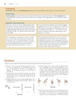
12. A circular ring of charge with radius b has total charge q
uniformly distributed around it. What is the magnitude of
the electric field at the center of the ring? (a) 0 (b) keq/b 2
(c) keq 2/b 2 (d) keq 2/b (e) none of those answers
13. Assume a uniformly charged ring of radius R and charge
Q produces an electric field E ring at a point P on its axis,
at distance x away from the center of the ring as in Figure OQ23.13a. Now the same charge Q is spread uniformly
over the circular area the ring encloses, forming a flat disk
of charge with the same radius as in Figure OQ23.13b.
How does the field E disk produced by the disk at P compare with the field produced by the ring at the same point?
(a) E disk , E ring (b) E disk 5 E ring (c) E disk . E ring (d) impossible to determine

Q
R
x

P

S

Ering
x

a
Q
R
x

P

S

Edisk
x

b

Figure OQ23.13
14. An object with negative charge is placed in a region of
space where the electric field is directed vertically upward.
What is the direction of the electric force exerted on this
charge? (a) It is up. (b) It is down. (c) There is no force.

(d) The force can be in any direction.
15. A free electron and a free proton are released in identical
electric fields. (i) How do the magnitudes of the electric
force exerted on the two particles compare? (a) It is millions of times greater for the electron. (b) It is thousands
of times greater for the electron. (c) They are equal. (d) It
is thousands of times smaller for the electron. (e) It is millions of times smaller for the electron. (ii) Compare the
magnitudes of their accelerations. Choose from the same
possibilities as in part (i).

denotes answer available in Student
Solutions Manual/Study Guide
What might happen if the personnel wore shoes with rubber soles?
3. A person is placed in a large, hollow, metallic sphere that
is insulated from ground. If a large charge is placed on


CHAPTER 23 | Electric Fields

682

the sphere, will the person be harmed upon touching the
inside of the sphere?
4. A student who grew up in a tropical country and is studying in the United States may have no experience with static
electricity sparks and shocks until his or her first American
winter. Explain.
5. If a suspended object A is attracted to a charged object B,
can we conclude that A is charged? Explain.
6. Consider point A in Figure
CQ23.6 located an arbitrary
distance from two positive

point charges in otherwise
empty space. (a) Is it possible for an electric field to
exist at point A in empty
space? Explain. (b) Does
charge exist at this point?
Explain. (c) Does a force
exist at this point? Explain.

A

ϩ

ϩ

Figure CQ23.6

7. In fair weather, there is an electric field at the surface of
the Earth, pointing down into the ground. What is the sign
of the electric charge on the ground in this situation?
8. A charged comb often attracts small bits of dry paper that
then fly away when they touch the comb. Explain why that
occurs.
9. A balloon clings to a wall after it is negatively charged by
rubbing. (a) Does that occur because the wall is positively
charged? (b) Why does the balloon eventually fall?
10. Consider two electric dipoles in empty space. Each dipole
has zero net charge. (a) Does an electric force exist between
the dipoles; that is, can two objects with zero net charge
exert electric forces on each other? (b) If so, is the force
one of attraction or of repulsion?

11. (a) Would life be different if the electron were positively
charged and the proton were negatively charged? (b) Does
the choice of signs have any bearing on physical and chemical interactions? Explain your answers.

Problems
denotes asking for quantitative and conceptual reasoning

The problems found in this chapter may be assigned
online in Enhanced WebAssign
1. denotes straightforward problem; 2. denotes intermediate problem;
3. denotes challenging problem
1. full solution available in the Student Solutions Manual/Study Guide

1. denotes problems most often assigned in Enhanced WebAssign;

denotes symbolic reasoning problem
denotes Master It tutorial available in Enhanced WebAssign
denotes guided problem

shaded denotes “paired problems” that develop reasoning with
symbols and numerical values

these provide students with targeted feedback and either a Master It
tutorial or a Watch It solution video.

helical molecule acts like a spring and compresses 1.00%
upon becoming charged. Determine the effective spring
constant of the molecule.

Section 23.1 Properties of Electric Charges

1. Find to three significant digits the charge and the mass of
the following particles. Suggestion: Begin by looking up the
mass of a neutral atom on the periodic table of the elements
in Appendix C. (a) an ionized hydrogen atom, represented
as H1 (b) a singly ionized sodium atom, Na1 (c) a chloride
ion Cl2 (d) a doubly ionized calcium atom, Ca11 5 Ca21
(e) the center of an ammonia molecule, modeled as an
N32 ion (f) quadruply ionized nitrogen atoms, N41, found
in plasma in a hot star (g) the nucleus of a nitrogen atom
(h) the molecular ion H2O2
2. (a) Calculate the number of electrons in a small, electrically neutral silver pin that has a mass of 10.0 g. Silver has
47 electrons per atom, and its molar mass is 107.87 g/mol.
(b) Imagine adding electrons to the pin until the negative
charge has the very large value 1.00 mC. How many electrons are added for every 109 electrons already present?

4. Nobel laureate Richard Feynman (1918–1988) once said
that if two persons stood at arm’s length from each other
and each person had 1% more electrons than protons,
the force of repulsion between them would be enough
to lift a “weight” equal to that of the entire Earth. Carry
out an order-of-magnitude calculation to substantiate this
assertion.
5.

A 7.50-nC point charge is located 1.80 m from a
4.20-nC point charge. (a) Find the magnitude of the electric force that one particle exerts on the other. (b) Is the
force attractive or repulsive?

6.

(a) Find the magnitude of the electric force between a
Na1 ion and a Cl2 ion separated by 0.50 nm. (b) Would the
answer change if the sodium ion were replaced by Li1 and
the chloride ion by Br2? Explain.

7.

(a) Two protons in a molecule are 3.80 3 10210 m
apart. Find the magnitude of the electric force exerted by
one proton on the other. (b) State how the magnitude of
this force compares with the magnitude of the gravitational
force exerted by one proton on the other. (c) What If? What

Section 23.2 Charging Objects by Induction
Section 23.3 Coulomb’s Law
3. Review. A molecule of DNA (deoxyribonucleic acid) is
2.17 mm long. The ends of the molecule become singly
ionized: negative on one end, positive on the other. The


| Problems
must be a particle’s charge-to-mass ratio if the magnitude
of the gravitational force between two of these particles is
equal to the magnitude of electric force between them?

y

q2

q3

ϩ

ϩ

Ϫ

0.500 m
60.0Њ
ϩ
2.00 mC

14.

Figure P23.8
9. Three point charges are arranged as shown in Figure
P23.9. Find (a) the magnitude and (b) the direction of the
electric force on the particle at the origin.
y
5.00 nC
ϩ
0.100 m
Ϫ
–3.00 nC

0.300 m

6.00 nC
x
ϩ

Figure P23.9
10. Two small metallic spheres, each of
mass m 5 0.200 g, are suspended as
pendulums by light strings of length L
as shown in Figure P23.10. The spheres
are given the same electric charge of
7.2 nC, and they come to equilibrium
when each string is at an angle of u 5
5.008 with the vertical. How long are
the strings?
11.

q1

q2
ϩ

L

m

θ

m

Figure P23.10

Particle A of charge 3.00 3 1024 C is at the origin,
particle B of charge 26.00 3 1024 C is at (4.00 m, 0), and

particle C of charge 1.00 3 1024 C is at (0, 3.00 m). We wish
to find the net electric force on C. (a) What is the x component of the electric force exerted by A on C? (b) What is
the y component of the force exerted by A on C? (c) Find
the magnitude of the force exerted by B on C. (d) Calculate the x component of the force exerted by B on C.
(e) Calculate the y component of the force exerted by B on
C. (f) Sum the two x components from parts (a) and (d) to
obtain the resultant x component of the electric force acting on C. (g) Similarly, find the y component of the resultant force vector acting on C. (h) Find the magnitude and
direction of the resultant electric force acting on C.

17.

A point charge 12Q is at
the origin and a point charge
2Q is located along the x axis
at x 5 d as in Figure P23.17.
Find a symbolic expression
for the net force on a third
point charge 1Q located
along the y axis at y 5 d.

x

d

Figure P23.11 Problems 11 and 12.

13.

Two small beads having charges q 1 and q 2 of the
same sign are fixed at the opposite ends of a horizontal

insulating rod of length d. The bead with charge q 1 is at the
origin. As shown in Figure P23.11, a third small, charged
bead is free to slide on the rod. (a) At what position x is
the third bead in equilibrium? (b) Can the equilibrium be
stable?
Three charged particles are located at the corners of
an equilateral triangle as shown in Figure P23.13. Calculate the total electric force on the 7.00-mC charge.

Review. Two identical particles,
y
each having charge 1q, are fixed in
ϩ
space and separated by a distance
ϩq
d. A third particle with charge 2Q
d
is free to move and lies initially at
2
ϪQ
rest on the perpendicular bisector
x
Ϫ
of the two fixed charges a distance
x
d
x from the midpoint between those
2
charges (Fig. P23.14). (a) Show that
if x is small compared with d, the
ϩ

ϩq
motion of 2Q is simple harmonic
along the perpendicular bisecFigure P23.14
tor. (b) Determine the period of
that motion. (c) How fast will the
charge 2Q be moving when it is at the midpoint between
the two fixed charges if initially it is released at a distance
a ,, d from the midpoint?

16.

x

12.

x

15. Review. In the Bohr theory of the hydrogen atom, an electron moves in a circular orbit about a proton, where the
radius of the orbit is 5.29 3 10211 m. (a) Find the magnitude of the electric force exerted on each particle. (b) If
this force causes the centripetal acceleration of the electron, what is the speed of the electron?

Two small beads having positive charges q 1 5 3q and
q 2 5 q are fixed at the opposite ends of a horizontal insulating rod of length d 5 1.50 m. The bead with charge q 1
is at the origin. As shown in Figure P23.11, a third small,
charged bead is free to slide on the rod. (a) At what position x is the third bead in equilibrium? (b) Can the equilibrium be stable?
ϩ

Ϫ

Ϫ4.00 mC

Figure P23.13 Problems 13 and 22.

d2

d1

7.00 mC
ϩ

8. Three point charges lie along a straight line as shown in
Figure P23.8, where q 1 5 6.00 mC, q 2 5 1.50 mC, and q 3 5
22.00 mC. The separation distances are d1 5 3.00 cm and
d 2 5 2.00 cm. Calculate the magnitude and direction of
the net electric force on (a) q 1, (b) q 2, and (c) q 3.
q1

683

y
ϩQ ϩ
d
ϩ
ϩ2Q

d

Ϫ
ϪQ

x

18. Why is the following situation
Figure P23.17
impossible? Two identical dust
particles of mass 1.00 mg are floating in empty space, far
from any external sources of large gravitational or electric


684

CHAPTER 23 | Electric Fields

fields, and at rest with respect to each other. Both particles
carry electric charges that are identical in magnitude and
sign. The gravitational and electric forces between the particles happen to have the same magnitude, so each particle
experiences zero net force and the distance between the
particles remains constant.
19. Two identical conducting small spheres are placed with
their centers 0.300 m apart. One is given a charge of
12.0 nC and the other a charge of 218.0 nC. (a) Find the
electric force exerted by one sphere on the other. (b) What
If? The spheres are connected by a conducting wire. Find
the electric force each exerts on the other after they have
come to equilibrium.
Section 23.4 The Electric Field
20. A small object of mass 3.80 g and charge 218.0 mC is suspended motionless above the ground when immersed in a
uniform electric field perpendicular to the ground. What
are the magnitude and direction of the electric field?
21.

In Figure P23.21,
1.00 m
determine the point (other
ϩ
Ϫ
than infinity) at which the
electric field is zero.
Ϫ2.50 mC
6.00 mC
22. Three charged particles
Figure P23.21
are at the corners of an
equilateral triangle as shown in Figure P23.13. (a) Calculate the electric field at the position of the 2.00-mC charge
due to the 7.00-mC and 24.00-mC charges. (b) Use your
answer to part (a) to determine the force on the 2.00-mC
charge.
23. Three point charges are located on a circular arc as shown
in Figure P23.23. (a) What is the total electric field at P, the
center of the arc? (b) Find the electric force that would be
exerted on a 25.00-nC point charge placed at P.
ϩ

ϩ3.00 nC

26.

30.0Њ
P

r

150°

ϩq
30°

x

270°

28.

PЈ
2d
ϩQ
Consider n equal positively charged particles each
Figure P23.27
of magnitude Q/n placed
symmetrically around a circle of radius a. (a) Calculate the
magnitude of the electric field at a point a distance x from
the center of the circle and on the line passing through
the center and perpendicular to the plane of the circle.
(b) Explain why this result is identical to the result of the
calculation done in Example 23.7.

ϩ

Section 23.5 Electric Field of a Continuous Charge Distribution
29. A rod 14.0 cm long is uniformly charged and has a total
charge of 222.0 mC. Determine (a) the magnitude and

(b) the direction of the electric field along the axis of the
rod at a point 36.0 cm from its center.
30. A uniformly charged disk of radius 35.0 cm carries charge
with a density of 7.90 3 1023 C/m2. Calculate the electric
field on the axis of the disk at (a) 5.00 cm, (b) 10.0 cm,
(c) 50.0 cm, and (d) 200 cm from the center of the disk.
31.

A uniformly charged ring of radius 10.0 cm has a total
charge of 75.0 mC. Find the electric field on the axis of the
ring at (a) 1.00 cm, (b) 5.00 cm, (c) 30.0 cm, and (d) 100 cm
from the center of the ring.

32.

Example 23.8 derives the exact expression for the
electric field at a point on the axis of a uniformly charged
disk. Consider a disk of radius R 5 3.00 cm having a uniformly distributed charge of 15.20 mC. (a) Using the result
of Example 23.8, compute the electric field at a point
on the axis and 3.00 mm from the center. (b) What If?
Explain how the answer to part (a) compares with the field
computed from the near-field approximation E 5 s/2P0.
(We will derive this expression in Chapter 24.) (c) Using
the result of Example 23.8, compute the electric field at a
point on the axis and 30.0 cm from the center of the disk.
(d) What If? Explain how the answer to part (c) compares
with the electric field obtained by treating the disk as a
15.20-mC charged particle at a distance of 30.0 cm.

33.

A continuous line of charge lies along the x axis,
extending from x 5 1x 0 to positive infinity. The line carries positive charge with a uniform linear charge density
l0. What are (a) the magnitude and (b) the direction of
the electric field at the origin?

34.

The electric field along the axis of a uniformly
charged disk of radius R and total charge Q was calculated

4.00 cm
ϩ3.00 nC

Figure P23.23
Two charged particles are located on the x
axis. The first is a charge 1Q at x 5 2a. The second is an
unknown charge located at x 5 13a. The net electric field
these charges produce at the origin has a magnitude of
2keQ/a 2. Explain how many values are possible for the unknown
a
ϩq
ϩ
charge and find the possible 2q
values.
25.
Four charged particles are at
a
a
the corners of a square of side a

as shown in Figure P23.25. Deter3q
4q
mine (a) the electric field at the
ϩ
ϩ
a
location of charge q and (b) the
total electric force exerted on q.
Figure P23.25

q ϩ

Two equal positively charged
Ϫ Ϫ2q
particles are at opposite corners of a trapezoid as shown in
Figure P23.26
Figure P23.27. Find symbolic
expressions for the total
d
P
ϩQ ϩ
electric field at (a) the point
P and (b) the point P9.
45.0Њ
45.0Њ

30.0Њ

ϩ

y

27.

4.00 cm
Ϫ2.00 nC
Ϫ

Three point charges lie
along a circle of radius r at
angles of 308, 1508, and 2708 as
shown in Figure P23.26. Find
a symbolic expression for the
resultant electric field at the
center of the circle.

24.


| Problems

35.

36.

37.

38.

685

in Example 23.8. Show that the electric field at distances
x that are large compared with R approaches that of a
particle with charge Q 5 spR 2. Suggestion: First show that
x/(x 2 1 R 2)1/2 5 (1 1 R 2/x 2)21/2 and use the binomial
expansion (1 1 d)n < 1 1 nd, when d ,, 1.

40. A positively charged disk has a uniform charge per unit
area s as described in Example 23.8.
Sketch the electric field lines in a
plane perpendicular to the plane of
the disk passing through its center.

A uniformly charged insulating rod
of length 14.0 cm is bent into the shape
of a semicircle as shown in Figure P23.35.
The rod has a total charge of 27.50 mC.
Find (a) the magnitude and (b) the direction of the electric field at O, the center of
the semicircle.

41. Figure P23.41 shows the electric field
lines for two charged particles separated by a small distance. (a) Determine the ratio q 1/q 2. (b) What are
the signs of q 1 and q 2?

O

42.

A uniformly charged rod of Figure P23.35
length L and total charge Q lies along the

x axis as shown in Figure
y
P23.36. (a) Find the components of the electric field at P
the point P on the y axis a
distance d from the origin.
d
(b) What are the approximate values of the field
x
components when d .. O
L
L? Explain why you would
expect these results.
Figure P23.36
A thin rod of length , and
uniform charge per unit length l
lies along the x axis as shown in
Figure P23.37. (a) Show that the
electric field at P, a distance d
from the rod along its perpendicular bisector, has no x component
and is given by E 5 2ke l sin u0 /d.
(b) What If? Using your result
to part (a), show that the field
of a rod of infinite length is E 5
2ke l/d.

y

u0
d

x

Figure P23.37

(a) Consider a uniformly charged, thin-walled, right
circular cylindrical shell having total charge Q, radius R,
and length ,. Determine the electric field at a point a distance d from the right side of the cylinder as shown in Figure P23.38. Suggestion: Use the result of Example 23.7 and
treat the cylinder as a collection of ring charges. (b) What
If? Consider now a solid cylinder with the same dimensions and carrying the same charge, uniformly distributed
through its volume. Use the result of Example 23.8 to find
the field it creates at the same point.

Figure P23.41
Pϩ
a

ϩ

q

q
a

a

ϩ

q

Figure P23.42

Section 23.7 Motion of a Charged Particle
in a Uniform Electric Field

44. A proton is projected in the positive
x direction into a region
S
of a uniform electric field E 5 1 26.00 3 105 2 i^ N/C at
t 5 0. The proton travels 7.00 cm as it comes to rest. Determine (a) the acceleration of the proton, (b) its initial speed,
and (c) the time interval over which the proton comes to
rest.
45.

A proton accelerates from rest in a uniform electric
field of 640 N/C. At one later moment, its speed is
1.20 Mm/s (nonrelativistic because v is much less than
the speed of light). (a) Find the acceleration of the proton. (b) Over what time interval does the proton reach
this speed? (c) How far does it move in this time interval?
(d) What is its kinetic energy at the end of this interval?

46.

Two horizontal metal plates, each 10.0 cm square, are
aligned 1.00 cm apart with one above the other. They are
given equal-magnitude charges of opposite sign so that a
uniform downward electric field of 2.00 3 103 N/C exists
in the region between them. A particle of mass 2.00 3
10216 kg and with a positive charge of 1.00 3 1026 C leaves
the center of the bottom negative plate with an initial speed
of 1.00 3 105 m/s at an angle of 37.08 above the horizontal.

(a) Describe the trajectory of the particle. (b) Which plate
does it strike? (c) Where does it strike, relative to its starting point?

47.

The electrons in a particle beam each have a kinetic
energy K. What are (a) the magnitude and (b) the direction of the electric field that will stop these electrons in a
distance d?

48.

Protons are projected with an initial speed vi 5
9.55 km/s from a field-free region through
a plane and into
S
a region where a uniform electric field E 5 2720j^ N/C is

,
R

q1

43. An electron and a proton are each placed at rest in a uniform electric field of magnitude 520 N/C. Calculate the
speed of each particle 48.0 ns after being released.

P

O
ᐉ

Three equal positive charges
q are at the corners of an equilateral triangle of side a as shown in
Figure P23.42. Assume the three
charges together create an electric
field. (a) Sketch the field lines in the
plane of the charges. (b) Find the
location of one point (other than `)
where the electric field is zero. What
are (c) the magnitude and (d) the
direction of the electric field at P
due to the two charges at the base?

q2

d
Q

Figure P23.38
Section 23.6 Electric Field Lines
39. A negatively charged rod of finite length carries charge
with a uniform charge per unit length. Sketch the electric
field lines in a plane containing the rod.


CHAPTER 23 | Electric Fields

686

present above the plane as shown in Figure P23.48. The
initial velocity vector of the protons makes an angle u with

the plane. The protons are to hit a target that lies at a horizontal distance of R 5 1.27 mm from the point where the
protons cross the plane and enter the electric field. We
wish to find the angle u at which the protons must pass
through the plane to strike the target. (a) What analysis
model describes the horizontal motion of the protons
above the plane? (b) What analysis model describes the vertical motion of the protons above the plane? (c) Argue that
Equation 4.13 would be applicable to the protons in this
situation. (d) Use Equation 4.13 to write an expression for
R in terms of vi , E, the charge and mass of the proton, and
the angle u. (e) Find the two possible values of the angle u.
(f) Find the time interval during which the proton is above
the plane in Figure P23.48 for each of the two possible values of u.
S

E ϭ Ϫ720ˆj N/C

field that enables the block to
Q
remain at rest. (b) If m 5
m
5.40 g, Q 5 27.00 mC, and u 5
25.08, determine the magniu
tude and the direction of the
electric field that enables the
block to remain at rest on
Figure P23.51
the incline.
52. Three solid plastic cylinders
all have radius 2.50 cm and length 6.00 cm. Find the charge
of each cylinder given the following additional information about each one. Cylinder (a) carries charge with uniform density 15.0 nC/m2 everywhere on its surface. Cylinder (b) carries charge with uniform density 15.0 nC/m2 on

its curved lateral surface only. Cylinder (c) carries charge
with uniform density 500 nC/m3 throughout the plastic.
53.
Consider an infinite number of identical particles,
each with charge q, placed along the x axis at distances a,
2a, 3a, 4a, . . . from the origin. What is the electric field at
the origin due to this distribution? Suggestion: Use

vi

u

؋ Target

54.

R
Proton
beam

S

E ϭ 0 below the plane

55.

Figure P23.48
49.

1

1
1
p2
1 2 1 2 1... 5
2
6
2
3
4
A particle with charge 23.00 nC is at the origin, and a particle with negative charge of magnitude Q is at x 5 50.0 cm.
A third particle with a positive charge is in equilibrium at
x 5 20.9 cm. What is Q?
A line of charge starts at x 5 1x 0 and extends to positive infinity. The linear charge density is l 5 l0x 0 /x, where
l0 is a constant. Determine the electric field at the origin.
Two small silver spheres, each with a mass of 10.0 g, are
separated by 1.00 m. Calculate the fraction of the electrons in one sphere that must be transferred to the other
to produce an attractive force of 1.00 3 104 N (about 1 ton)
between the spheres. The number of electrons per atom of
silver is 47.
A uniform electric field of magnitude 640 N/C exists
between two parallel plates that are 4.00 cm apart. A proton is released from rest at the positive plate at the same
instant an electron is released from rest at the negative
plate. (a) Determine the distance from the positive plate at
which the two pass each other. Ignore the electrical attraction between the proton and electron. (b) What If? Repeat
part (a) for a sodium ion (Na1) and a chloride ion (Cl2).
Two point charges qA 5 212.0 mC and q B 5 45.0 mC
and a third particle with unknown charge q C are located on
the x axis. The particle qA is at the origin, and q B is at x 5
15.0 cm. The third particle is to be placed so that each particle is in equilibrium under the action of the electric forces
exerted by the other two particles. (a) Is this situation possible? If so, is it possible in

S
u
more than one way? Explain.
E
y
Find (b) the required location and (c) the magnitude
x
and the sign of the charge of
ϩ
the third particle.
q
A charged cork ball of
mass 1.00 g is suspended on a
Figure P23.59
light string in the presence of a
Problems 59 and 60.
uniform electric field as shown
11

S

A proton moves at 4.50 3 105 m/s in the horizontal
direction. It enters a uniform vertical electric field with a
magnitude of 9.60 3 103 N/C. Ignoring any gravitational
effects, find (a) the time interval required for the proton
to travel 5.00 cm horizontally, (b) its vertical displacement
during the time interval in which it travels 5.00 cm horizontally, and (c) the horizontal and vertical components of
its velocity after it has traveled 5.00 cm horizontally.

56.

57.

Additional Problems
50. A small sphere of charge
q 1 5 0.800 mC hangs from
the end of a spring as in
Figure P23.50a. When
another small sphere of
charge q 2 5 20.600 mC
is held beneath the first
sphere as in Figure P23.50b,
the spring stretches by d 5
3.50 cm from its original
length and reaches a new
equilibrium position with
a separation between the
charges of r 5 5.00 cm.
What is the force constant
of the spring?

k

k
ϩ
q1

58.

ϩ

d
r

Ϫ
q2
a

b

Figure P23.50

51. A small block of mass m and charge Q is placed on an insulated, frictionless, inclined plane of angle u as in Figure
P23.51. An electric field is applied parallel to the incline.
(a) Find an expression for the magnitude of the electric

59.


| Problems
in Figure P23.59. When E 5 1 3.00 i^ 1 5.00 j^ 2 3 105 N/C,
the ball is in equilibrium at u 5 37.08. Find (a) the charge
on the ball and (b) the tension in the string.
S

60.

A charged cork ball of mass m is suspended on a light
string in the presence of S
a uniform electric field as shown

in Figure P23.59. When E 5 A i^ 1 B j^ , where A and B are
positive numbers, the ball is in equilibrium at the angle u.
Find (a) the charge on the ball and (b) the tension in the
string.

charge 1200 nC. Find the distance between the centers of
the spheres.
66. Three identical point charges, each of mass m 5 0.100 kg,
hang from three strings as shown in Figure P23.66. If the
lengths of the left and right strings are each L 5 30.0 cm
and the angle u is 45.08, determine the value of q.

θ

61. Three charged particles are aligned along the x axis as
shown in Figure P23.61. Find the electric field at (a) the
position (2.00 m, 0) and (b) the position (0, 2.00 m).

Ϫ

ϩq

Ϫ4.00 nC

0.800 m
ϩ

ϩ

ϩq

W

q

ϩ

L

ϩ
m

ϩq

67. Review. Two identical blocks resting on a frictionless, horizontal surface are connected by a light spring having a
spring constant k 5 100 N/m and an unstretched length
L i 5 0.400 m as shown in Figure P23.67a. A charge Q is
slowly placed on each block, causing the spring to stretch
to an equilibrium length L 5 0.500 m as shown in Figure
P23.67b. Determine the value of Q , modeling the blocks as
charged particles.

y
q ϩ

ϩ
m

Figure P23.66

Figure P23.61

62. Four identical charged particles (q 5 110.0 mC) are located
on the corners of a rectangle as
shown in Figure P23.62. The
dimensions of the rectangle are
L 5 60.0 cm and W 5 15.0 cm.
Calculate (a) the magnitude
and (b) the direction of the
total electric force exerted on
the charge at the lower left corner by the other three charges.

L

ϩq

ϩ
m

x

3.00 nC

5.00 nC

θ

L

y
0.500 m

687

Li
k

ϩ x
q

Figure P23.62

63. A line of positive charge is
y
formed into a semicircle
of radius R 5 60.0 cm as
shown in Figure P23.63.
u
The charge per unit length
R
along the semicircle is
described by the expresP
sion l 5 l0 cos u. The total
charge on the semicircle
is 12.0 mC. Calculate the
Figure P23.63
total force on a charge of
3.00 mC placed at the center of curvature P.

a
Q

L
k

Q

b

Figure P23.67 Problems 67 and 68.
x

64. Why is the following situation impossible? An electron enters
a region of uniform electric field between two parallel
plates. The plates are used in a cathode-ray tube to adjust
the position of an electron beam on a distant fluorescent
screen. The magnitude of the electric field between the
plates is 200 N/C. The plates are 0.200 m in length and
are separated by 1.50 cm. The electron enters the region
at a speed of 3.00 3 106 m/s, traveling parallel to the plane
of the plates in the direction of their length. It leaves the
plates heading toward its correct location on the fluorescent screen.
65. Two small spheres hang in equilibrium at the bottom ends
of threads, 40.0 cm long, that have their top ends tied to
the same fixed point. One sphere has mass 2.40 g and
charge 1300 nC. The other sphere has the same mass and

68.

Review. Two identical blocks resting on a frictionless,
horizontal surface are connected by a light spring having a
spring constant k and an unstretched length L i as shown in

Figure P23.67a. A charge Q is slowly placed on each block,
causing the spring to stretch to an equilibrium length L as
shown in Figure P23.67b. Determine the value of Q, modeling the blocks as charged particles.
69. Two hard rubber spheres,
d
each of mass m 5 15.0 g,
are rubbed with fur on
a dry day and are then
L
suspended with two insuu
u
lating strings of length
L 5 5.00 cm whose supm
m
port points are a distance
d 5 3.00 cm from each
Figure P23.69
other as shown in Figure
P23.69. During the rubbing process, one sphere receives
exactly twice the charge of the other. They are observed to
hang at equilibrium, each at an angle of u 5 10.08 with the
vertical. Find the amount of charge on each sphere.


688
70.

71.

CHAPTER 23 | Electric Fields

Show that the maximum magnitude E max of the electric
field along the axis of a uniformly charged ring occurs at x 5
a/ !2 (see Fig. 23.16) and has the value Q / 1 6!3pP0a 2 2 .
Two small spheres of mass m are suspended
from strings of length , that are connected at a common
point. One sphere has charge Q and the other charge
2Q. The strings make angles u1 and u2 with the vertical.
(a) Explain how u1 and u2 are related. (b) Assume u1 and u2
are small. Show that the distance r between the spheres is
approximately
r
4k eQ2 ,
mg

1/3

b

72.

Two identical beads
each have a mass m and
R
R
charge q. When placed in
a hemispherical bowl of
m
m

d
ϩ
ϩ
radius R with frictionless,
nonconducting walls, the
beads move, and at equilibrium, they are a disFigure P23.72
tance d apart (Fig. P23.72).
(a) Determine the charge
q on each bead. (b) Determine the charge required for d to
become equal to 2R.

73.

Review. A 1.00-g cork ball with charge 2.00 mC is
suspended vertically on a 0.500-m-long light string in
the presence of a uniform, downward-directed electric
field of magnitude E 5 1.00 3 105 N/C. If the ball is displaced slightly from the vertical, it oscillates like a simple
pendulum. (a) Determine the period of this oscillation.
(b) Should the effect of gravitation be included in the calculation for part (a)? Explain.

74.

y
b
Ϫa

b Ϫa

a

b ϩa

x

Figure P23.75
76. Inez is putting up decorations for her sister’s
quinceañera (fifteenth
birthday party). She ties
three light silk ribbons
together to the top of a
gateway and hangs a rubber balloon from each
ribbon (Fig. P23.76). To
include the effects of the
gravitational and buoyant forces on it, each balloon can be modeled as
Figure P23.76
a particle of mass 2.00 g,
with its center 50.0 cm
from the point of support. Inez rubs the whole surface of
each balloon with her woolen scarf, making the balloons
hang separately with gaps between them. Looking directly
upward from below the balloons, Inez notices that the
centers of the hanging balloons form a horizontal equilateral triangle with sides 30.0 cm long. What is the common
charge each balloon carries?
77.

Review. A negatively
Q
charged particle 2q is
placed at the center of a
a

uniformly charged ring,
where the ring has a total
positive charge Q as shown
Ϫq
x
in Figure P23.74. The particle, confined to move
along the x axis, is moved
a small distance x along
Figure P23.74
the axis (where x ,, a)
and released. Show that
the particle oscillates in simple harmonic motion with a
frequency given by

Eight charged particles, each of magnitude q, are
located on the corners of a cube of edge s as shown in Figure P23.77. (a) Determine the x, y, and z components of
the total force exerted by the other charges on the charge
located at point A. What are (b) the magnitude and (c) the
direction of this total force?
z
q
q
q

q

Point
A

q

s
s

q
x

q

y

s
q

1 k eqQ 1/2
f5
a
b
2p ma 3
Challenge Problems
75.

Identical thin rods of length 2a carry equal charges
1Q uniformly distributed along their lengths. The rods lie
along the x axis with their centers separated by a distance
b . 2a (Fig. P23.75). Show that the magnitude of the force
exerted by the left rod on the right one is
F5a

k eQ

4a

2

2

b ln a

b2
b
b 2 4a 2
2

Figure P23.77 Problems 77 and 78.
78.

Consider the charge distribution shown in Figure
P23.77. (a) Show that the magnitude of the electric field at
the center of any face of the cube has a value of 2.18keq/s 2.
(b) What is the direction of the electric field at the center
of the top face of the cube?

79.

Review. An electric dipole in a uniform horizontal
electric field is displaced slightly from its equilibrium position as shown in Figure P23.79, where u is small. The separation of the charges is 2a, and each of the two particles


| Problems
has mass m. (a) Assuming the dipole is released from this

position, show that its angular orientation exhibits simple
harmonic motion with a frequency
f5

qE
1
2pÅ ma

What If? (b) Suppose the masses of the two charged particles in the dipole are not the same even though each
particle continues to have charge q. Let the masses of the
particles be m1 and m 2. Show that the frequency of the
oscillation in this case is
f5

80.

1 qE 1 m 1 1 m 2 2
2pÅ 2am 1m 2

2a

u

Ϫq Ϫ

Figure P23.79

S

E

Two particles, each with charge 52.0 nC, are located
on the y axis at y 5 25.0 cm and y 5 225.0 cm. (a) Find
the vector electric field at a point on the x axis as a function of x. (b) Find the field at x 5 36.0 cm. (c) At what
location is the field 1.00i^ kN/C? You may need a computer
to solve this equation. (d) At what location is the field
16.0i^ kN/C?

81. A line of charge with uniform density 35.0 nC/m lies along
the line y 5 215.0 cm between the points with coordinates
x 5 0 and x 5 40.0 cm. Find the electric field it creates at
the origin.
82.

ϩ q

689

A particle of mass m and charge q moves at high speed
along the x axis. It is initially near x 5 2`, and it ends up
near x 5 1`. A second charge Q is fixed at the point x 5 0,
y 5 2d. As the moving charge passes the stationary charge,
its x component of velocity does not change appreciably,
but it acquires a small velocity in the y direction. Determine
the angle through which the moving charge is deflected
from the direction of its initial velocity.