Studies in Avian Biology 17

DEMOGRAPHY OF THE
NORTHERN SPOTTED OWL
ERIC D. FORSMAN, STEPHEN DESTEFANO,
MARTIN G. RAPHAEL, AND R. J. GUTIfiRREZ,

EDITORS

Studiesin Avian BiologyNo. 17
A Publicationof the CooperOrnithologicalSociety


DEMOGRAPHY
OF THE
NORTHERN
SPOTTED OWL
Eric D. Forsman,StephenDeStefano,
Martin G. Raphael,and R. J. Gutik-rez, editors

Proceedings
of a Workshop
Fort Collins,Colorado,
December1993

Sponsor:
USDA ForestService

Studies in Avian Biology No. 17
A PUBLICATION

OF THE COOPER ORNITHOLOGICAL

Cover drawing of Northern SpottedOwl by Viktor Bahktin

SOCIETY


STUDIES IN AVIAN BIOLOGY
Edited by
John T. Rotenberry
Department of Biology
University of California
Riverside, California 92 52 1

Studiesin AvianBiologyis a seriesof works too long for The Condor,published at irregular intervals by the Cooper Ornithological Society. Manuscripts
for consideration should be submitted to the editor. Style and format should
follow those of previous issues.
Price $20.00 including postageand handling. All orders cash in advance; make
checks payable to Cooper Ornithological Society. Send orders to Cooper Omithological Society, % Western Foundation of Vertebrate Zoology, 439 Calle San
Pablo, Camarillo, CA 93010.
ISBN: O-935868-83-6
Library of CongressCatalog Card Number: 96-085058
Printed at Allen Press,Inc., Lawrence, Kansas 66044
Issued: 26 June 1996
Copyright 0 by the Cooper Ornithological Society 1996


CONTENTS
LIST OF AUTHORS
PREFACE

..............................................

. . . . . . . . . . . . . . . . . . . . . . . . . . . . . . . . . . . . . . . . . . The Editors

INTRODUCTION

AND

V

1

METHODS

Biology and distribution of the Northern Spotted Owl . . R. J. Gutierrez
History of demographic studies in the management of the Northern Spotted Owl . . . . . . R. J. Gutierrez, Eric D. Forsman, Alan B. Franklin,
and E. Charles Meslow
Methods for collecting and analyzing demographic data on the Northern
Spotted Owl . . . . . . . . . . . . Alan B. Franklin, David R. Anderson,
Eric D. Forsman, Kenneth P. Bumham, and Frank W. Wagner
DEMOGRAPHY

OF THE NORTHERN

SPOTTED

12

OWL

Olympic Peninsula and east slope of the Cascade Range, Washington . .

. . . . . . . . . . . . . . Eric D. Forsman, Stan G. Sovem, D. Erran Seaman,
Kevin J. Maurice, Margaret Taylor, and Joseph J. Zisa

21

Salem District, Bureau of Land Management, Oregon . . . . . . . . . . . . . . . .
D. Scott Hopkins, Wayne D. Logan, and Eric D. Forsman
.. . ...

31

H. J. Andrews Experimental Forest and vicinity, Oregon . . . . . . . . . . . .
. . . . . . . . . . . . . Gary S. Miller, Stephen DeStefano, Keith A. Swindle,
and E. Charles Meslow

37

Siuslaw National Forest, Oregon . . . . Eric D. Forsman, Peter J. Loschl,
Raymond K. Forson, and Douglas K. Barrett

47

Eugene District, Bureau of Land Management, Oregon . . . . . . . . . . . . . .
. . . . . . . . . . . James A. Thrailkill, E. Charles Meslow, John P. Perkins,
and Lawrence S. Andrews

53

Roseburg District, Bureau of Land Management, Oregon . . . . . . . . . . . .
. . . . . . . . . . . . . Janice A. Reid, Eric D. Forsman, and Joseph B. Lint

59

Southern Cascades and Siskiyou Mountains, Oregon . . . . . . . . . . . . _. . . .
. . . . . . . . . Frank F. Wagner, E. Charles Meslow, Gregory M. Bennett,
Chris J. Larson, Stephen M. Small, and Stephen DeStefano

67

Coastal mountains of southwestern Oregon . . . . . . . . . . . . . . . . . . . . . . . . . .
. . . . . . . . . . . . . Cynthia J. Zabel, Susan E. Salmons, and Mark Brown

77

Northwestern California . . . . . . . . . . . Alan B. Franklin, R. J. Gutierrez,
Barry R. Noon, and James P. Ward, Jr.

83

SYNTHESIS
Meta-analysis of vital rates of the Northern Spotted Owl . . . . . . . . . . . . .
. . . . . Kenneth P. Bumham, David R. Anderson, and Gary C. White

92

Use, interpretation, and implications of demographic analyses of Northern
Spotted Owl populations . . Martin G. Raphael, Robert G. Anthony,
Stephen DeStefano, Eric D. Forsman, Alan B. Franklin,
Richard Holthausen, E. Charles Meslow, and Barry R. Noon

102

LITERATURE
APPENDIX-

............................................

113

Symbols and Acronyms . . . . . . . . . . . . . . . _. . . . . . . . . . . . . . .

121

CITED


LIST OF AUTHORS
DAVID R. ANDERSON
Colorado Cooperative Fish and Wildlife
ResearchUnit
National Biological Service
Colorado State University
Fort Collins, CO 80523

LAWRENCE
S. ANDREWS
Oregon Cooperative Wildlife ResearchUnit
104 Nash Hall
Oregon State University
Corvallis, OR 97330

ROBERTG. ANTHONY
National Biological Service
Oregon Cooperative Wildlife ResearchUnit
Oregon State University
Corvallis, OR 97330
DOUGLASK. BARRFIT
USDA Forest Service
Pacific Northwest ResearchStation
3200 SW JeffersonWay
Corvallis, OR 9733 1
GREGORYM. BENNETT
Oregon Cooperative Wildlife ResearchUnit
Department of Fisheries and Wildlife
Oregon State University
Corvallis, OR 97331
MARK BROWN
Arizona Game and Fish Department
9 140 East County 10% Street
Yuma. AZ 85365
KENNETHP. BURNHAM
Colorado Cooperative Fish and Wildlife
Research Unit
National Biological Service
Colorado State University
Fort Collins, CO 80523

RAYMONDK. FORSON
USDA Forest Service
Pacific Northwest ResearchStation
3200 SW JeffersonWay

Corvallis, OR 9733 1
ALAN B. FRANKLIN
Colorado Cooperative Fish and Wildlife
ResearchUnit
Department of Fishery and Wildlife Biology
Colorado State University
Fort Collins, CO 80523
R. J. GUTIBRREZ
Department of Wildlife
Humboldt State University
Arcata, CA 95521
D. SCOTTHOPKINS
USDI Bureau of Land Management
Salem District Office
17 17 Fabry Road
Salem, OR 97306
RICHARDHOLTHAUSEN
USDA Forest Service
104 Nash Hall
Oregon State University
Corvallis, OR 9733 1
CHRISJ. LARsON
Oregon Cooperative Wildlife ResearchUnit
Department of Fisheries and Wildlife
Oregon State University
Corvallis, OR 9733 1
JOSEPH
B. LINT
USDI Bureau of Land Management
777 Garden Valley Blvd.

Roseburg,OR 97470
WAYNED. LOGAN
USDI Bureau of Land Management
Salem District Office
17 17 Fabry Road
Salem. OR 97306

STEPHEN
DESTEFANO
Oregon Cooperative Wildlife ResearchUnit
Department of Fisheries and Wildlife
Oregon State University
Corvallis, OR 97330
(present address:National Biological Service
Coonerative Fish and Wildlife ResearchUnit
104 Biological SciencesEast
University of Arizona
Tucson, AZ 8527 1)

PETERJ. L~~CHL
USDA Forest Service
Pacific Northwest ResearchStation
3200 SW JeffersonWay
Corvallis, OR 9733 1

ERIC D. FORSMAN
USDA Forest Service
Pacific Northwest ResearchStation
3200 SW JeffersonWay
Corvallis, OR 9733 1

KEVIN J. MAURICE
USDA Forest Service
Pacific Northwest ResearchStation
3200 SW JeffersonWay
Corvallis, OR 9733 1


E. CHARLESMns~ow
National Biological Service
Oregon Cooperative Wildlife ResearchUnit
Oregon State University
Corvallis, OR 97330
(present address:Wildlife Management
Institute
8035 NW Oxbow Dr.
Corvallis, OR 97330)
GARY S. MILLER
Oregon Cooperative Wildlife ResearchUnit
Department of Fisheries and Wildlife
Oregon State University
Corvallis, OR 97331
(present address:US Fish and Wildlife Service
2600 SE 98th Ave.. Suite 100
Portland, OR 97266)
BARRYR. NCI~N
USDA Forest Service
Redwood SciencesLaboratory
1700 Bayview Dr.
Arcata, CA 95521

JOHNP. PERKINS
Oregon Cooperative Wildlife ResearchUnit
104 Nash Hall
Oregon State University
Corvallis, OR 97330
MARTIN G. RAPHAEL
USDA Forest Service
Pacific Northwest Research Station
3625 93rd Ave. SW
Olympia, WA 985 12
JANICEA. REID
USDA Forest Service
Pacific Northwest ResearchStation
RoseburgField Office
777 Garden Valley Blvd.
Roseburg,OR 97470

STEPHEN
M. SMALL
Oregon Cooperative Wildlife ResearchUnit
Department of Fisheries and Wildlife
Oregon State University
Corvallis, OR 9733 1
STANG. SOVERN
USDA Forest Service
Pacific Northwest ResearchStation
3200 SW JeffersonWay
Corvallis, OR 9733 1
KEITH A. SWINDLE
Oregon Cooperative Wildlife ResearchUnit

Department of Fisheries and Wildlife
Oregon State University
Corvallis, OR 97330
MARGARETTAYLOR
USDA Forest Service
Pacific Northwest ResearchStation
3200 SW JeffersonWay
Corvallis, OR 97331
JA~VIES
A. THRAIWLL
Oregon Cooperative Wildlife ResearchUnit
104 Nash Hall
Oregon State University
Corvallis, OR 97330
FRANKF. WAGNER
Oregon Cooperative Wildlife ResearchUnit
Department of Fisheries and Wildlife
Oregon State University
Corvallis, OR 9733 1
JAMESP. WARD, JR.
Department of Biology
Colorado State University
Fort Collins, CO 80523
GARY C. WHITE
Department of Fishery and Wildlife Biology
Colorado State University
Fort Collins, CO 80523

SUSANE. SALMONS
USDA Forest Service

Pacific SouthwestForest and Range
Experiment Station
1700 Bayview Dr.
Arcata. CA 95521

J. -EL
USDA Forest Service
Pacific SouthwestForest and Range
Experiment Station
1700 Bayview Dr.
Arcata, CA 95521

D. ERRANSEAMAN
National Biological Service
Olympic Field Unit
600 E. Park Ave.
Port Angeles, WA 98362

JOSEPH
J. ZISA
USDA Forest Service
Pacific Northwest ResearchStation
3200 SW JeffersonWay
Corvallis, OR 9733 1

CYNTHIA


Studies in Avian Biology No. 17: 1, 1996.

PREFACE
A large number of mark-recapture studies of
Northern Spotted Owls (Strix occidentalis caurina) were initiated during 1985-1990, with the
primary objective of evaluating trends in vital
rates of the species. These studies were conducted by scientists from federal agencies, universities, private timber companies, and consulting firms, and involved repeated surveys of
large areas each year to locate, mark, and reobserve or recapture resident pairs of owls and their
offspring. Some studies also included radiotelemetry to examine movements ofjuvenile owls.
At the request of the United States Secretaries
of Agriculture and Interior, a workshop was convened in Fort Collins, Colorado in December
1993 to examine all existing demographic data
on the Northern Spotted Owl. The workshop focused exclusively on mark-recapture studies, and
was led by Drs. K. P. Bumham, D. R. Anderson
and G. C. White. A number of other scientists
and analysts familiar with demographic analyses
were invited to participate in developing the analytical framework and assisting with data analysis.
Invited participants included all researchers
with three or more years of demographic data
on Northern Spotted Owls, including researchers
from seven studies conducted by federal agencies, two studies conducted by forest products
companies, four studies conducted by university
scientists, and one study conducted by a consulting company. The two forest products companies declined to present their data for analysis.
The consulting firm presented their data for analysis but withdrew their results at the end of the
workshop because they were not convinced that
their data met the underlying assumptions of the

capture-recapture models used in estimating survival probabilities. Thus, results of 11 studies
conducted by federal and university scientists
were the focus of the final workshop report.
The initial product of the Fort Collins workshop was a summary report prepared and submitted to the U. S. Departments of Agriculture
and Interior by the workshop leaders. That report was included as an appendix in agency planning documents (Bumham et al. 1994). Workshop participants felt that a more complete exposition of the workshop proceedings was appropriate, and agreed to prepare individual

reports on each of the 11 study areas for publication in a peer-reviewed journal. In addition to
the individual study area reports, several additional supporting papers were written, including
papers on the history of the issue, general biology
of the owl, methods, habitat trends, and management implications. The papers in this volume
represent the culmination of this effort.
We would like to thank the editors and reviewers at the Journal of Wildrife Management
for the very thorough and helpful reviews that
they provided on many of the manuscripts in
this report. Editor L. M. Smith, and Associate
Editors M. J. Conroy and W. R. Clark were instrumental in this regard. We also thank all those
who assisted with data analysis at the Fort Collins Workshop, including D. R. Anderson, K. P.
Bumham, J. Clobert, J. E. Hines, J. D. Nichols,
R. J. Pradel, E. A. Rexstad, T. M. Shenk, G. C.
White, and K. R. Wilson. Viktor Bakhtin of the
International Crane Foundation provided the
cover art.
THE EDITORS


Studies in Avian Biology No. 17:2-5, 1996.

BIOLOGY AND DISTRIBUTION
NORTHERN
SPOTTED OWL

OF THE

R. J. GUTI~REZ

INTRODUCTION

REGIONAL DISTRIBUTION

The Northern Spotted Owl (Striw occidentalis
caurina) is one of three subspeciesof the Spotted
Owl inhabiting western North America (Gutitrrez et al. 1995). The taxonomic separation of
these subspecies is supported by genetic (Barrowclough and Gutierrez 1990, G. Barrowclough, personal communication), morphological (Gutitrrez et al. 1995), and biogeographic
information (Barrowclough and Gutierrez 1990).
The purpose of this chapter is to provide a
synopsis of relevant biology of the Northern
Spotted Owl particularly with respect to its distribution, habitat use, and life history characteristics. Other literature reviews of Spotted Owl
biology that are particularly comprehensive include Campbell et al. (1984), Gutietrez (1985),
Gutierrez and Carey (1985), Thomas et al. (1990)
Vemer et al. (1992) and Gutierrez et al. (1995).

The distribution of the Northern Spotted Owl
within its known range is relatively contiguous,
but is influenced by the natural insularity of habitat patches within geographic provinces, and by
natural and man-caused fragmentation of vegetation within and among geographic provinces.
For example, few Spotted Owls occur in the westem Washington Lowlands where nearly all old
forests have been logged and replaced with young
forests (USDI 1992a, Gutierrez 1994a). As a result of the natural and man-caused fragmentation of habitat, Spotted Owls may exhibit a metapopulation structure in some parts of their range
(Gutierrez and Harrison in press).

PHYSICAL

BEHAVIOR
Spotted Owls are territorial. However, the fact
that home ranges of adjacent pairs overlap (Forsman et al. 1984, Solis and Gutierrez 1990) suggests that the area defended is smaller than the
areas used for foraging. Territorial defense is primarily effected by hooting calls, barking calls,

and/or shrill whistles (Forsman et al. 1984, Fitton 199 1). Because they respond readily to imitations of their calls, Spotted Owls are relatively
easy to locate (Forsman 1983, Franklin et al. this

DESCRIPTION

The Spotted Owl is a medium-sized owl, about
46-48 cm in length and weighs approximately
490-850 g (Dawson 1923, Hamer et al. 1994,
Gutierrez et al. 1995). The Northern Spotted Owl
is the largest of the three subspecies (Gutierrez
et al. 1995). It is dark brown with a barred tail
and white spots on the head and breast, and has
dark brown eyes that are surrounded by prominent facial disks (Bent 1938, Gutierrez et al.
1995). Three age classescan be distinguished on
the basis of plumage characteristics (Forsman
1981, Moen et al. 1991).
The Spotted Owl superficially resembles the
Barred Owl (Strix varia), a species with which it
occasionally hybridizes. Hybrids exhibit characteristics of both species (Hamer et al. 1994).

volume).
Northern Spotted Owls are monogamous and
usually form long-term pair bonds. “Divorces”
occur but are relatively uncommon. There are
no known examples of polygyny in this owl, although associations of 3 or more birds have been
reported (Forsman et al. 1984, Gutierrez et al.
1995). Males and females divide nesting duties,
with the male providing food to nesting females.
The female does all of the incubating and brooding of owlets (Forsman 1976).
Median home range sizes of Northern Spotted

Owls range from 5.7-40.2 km2 for owl pairs and
3.4-38.2 km2 for individual owls (see summary
in Gutierrez et al. 1995). Home range size appears to be correlated with the amount of habitat
fragmentation, suitable habitat, and/or primary
prey (Carey et al. 1992, Zabel et al. 1995). Spotted Owls maintain smaller home ranges during
the breeding season and often dramatically increase their home range size during fall and winter (Forsman 1980, Forsman et al. 1984, Sisco
1990).

DISTRIBUTION
GEOGRAPHICRANGE
The Northern Spotted Owl occurs in the
mountains of northwestern California (from
Marin Co. north), western Oregon, western
Washington, and southwestern British Columbia. The eastern edge of its range generally corresponds with the eastern periphery of the Cascades Range, and with the Central Valley in California (Bent 1938, Gutierrez et al. 1995).
2


BIOLOGY
HABITAT

OF THE NORTHERN

RELATIONSHIPS

HABITAT USE
Northern Spotted Owls have been detected in
many different forest habitats. Forsman et al.
(1984) reported owls from the following forest
types: Douglas-fir (Pseudotsugamenziesii), westem hemlock (Tsuga heterophylla),grand fir (Abies
grandis), white fir (A. concolor), ponderosa pine

(Pinus ponderosa), and Shasta red fir (A. magni$ca shastensis).Owls also have been recorded
using redwood (Sequoia sempervirens),western
red cedar (Thuja plicata), mixed conifer-hardwood (Klamath montane), and mixed evergreen
forest (Grinnell and Miller 1944, Forsman et al.
1984, LaHaye 1988, Solis and Gutitrrez 1990,
Folliard 1993). In essence, most low and midelevation conifer or conifer/hardwood forest types
within the subspecies’ range have been used by
the owl if they have the appropriate structure
(see below). Some owls have used pure hardwood
stands in the southern part of the range if a perennial water source was present.
In California, owls are found from near sea
level in coastal forests to a little over 2 130 m in
the Cascades. The upper elevational limits at
which Spotted Owls occur decreasegradually with
increasing latitude in Oregon and Washington.
In northern Washington and southern British
Columbia, few owls occur above 1500 m elevation. In all areas, the upper elevation limits at
which owls occur correspond to the transition to
subalpine forest, which is characterized by relatively simple structure and severe winter weather.
HABITAT SELECTION
Studies of habitat use indicate that Northern
Spotted Owls generally select mature and oldgrowth forest equal to or more than expected,
and early seral stage forest less than expected
(Forsman 1980, Forsman et al. 1984, Solis and
Gutiirrez 1990, Sisco 1990, Carey et al. 1990,
1992). Individual owls may show variation in
the general pattern, with some owls using intermediate-aged stands (SO-100 yrs old) in proportion to, or more than, expected. Several landscape level studies indicate that Northern Spotted Owls select habitats that have a significantly
higher proportion of mature/old-growth forests
around nests and roosts than is randomly available (Ripple et al. 199 1, Lemkuhl and Raphael
1993, Hunter et al. 1995).

Ward (1990) found that Spotted Owls foraged
in areas that had lower variance in prey densities
(prey were more predictable in occurrence) within older forest and near ecotones of old forest
and younger brush seral stages. Presumably owls
foraging in edge areas might encounter prey that

SPOTTED

OWL-

Gutikrez

3

ventured into the older forest. Carey et al. (1992)
and Carey and Peeler (1995) found that owls
occupying fragmented landscapes had larger
home ranges. When prey communities were
dominated by flying squirrels (Glaucomyssabrinus), Spotted Owls apparently depleted some local flying squirrel populations (Carey et al. 1992).
Carey et al. (1992) suggested that Spotted Owls
not only have to forage within many patches but
must also “monitor” prey recovery within depleted patches to efficiently use their home ranges. Finally, Zabel et al. (1995) showed that
Northern Spotted Owl home ranges are larger
where flying squirrels are the predominant prey
and, conversely, are smaller where woodrats (Neotoma spp.) are the predominant prey.

Habitat structure
Spotted Owls select roosts that have more
complex vegetation structure than forests generally available to them (Forsman 1976, Barrows
and Barrows 1978, Forsman 1980, Solis 1983,

Forsman et al. 1984, Chavez-Leon 1989, Sisco
1990, Solis and Gutierrez 1990). These habitats
are usually multi-layered forests having high canopy closure and large diameter trees in the overstory. In northwestern California, roosts usually
are found on the lower third of slopesnear streams
(Blakesley et al. 1992). Complex vegetation or
association with streams may facilitate thermoregulation by maintaining lower ambient stand
temperature and providing a variety of perch
sites which may allow owls to select cooler microclimates (Forsman 1976, Barrows and Barrows 1978, Barrows 1981, Solis 1983, Forsman
et al. 1984).
Northern Spotted Owls nest almost exclusively in trees. Like roosts, nest sites are found in
forests having complex structure dominated by
large diameter trees (Forsman et al. 1984, LaHaye
1988). Even in forests that have been previously
logged, owls select forests having a structure (i.e.,
larger trees, greater canopy closure) different than
forestsgenerally available to them (Folliard 1993,
Buchanan et al. 1995). Nests are usually platforms (e.g., old raptor nests, debris accumulations), or cavities in large trees. The proportion
of nest types used apparently is related to availability; platforms comprise a higher proportion
of nests in disturbed or young forests, whereas
nests in tree cavities tend to predominate in old
forests (Forsman et al. 1984, LaHaye 1988, Buchanan et al. 1993, Folliard 1993).
Foraging habitat is the most variable of all
habitats used by territorial owls (Thomas et al.
1990). Yet foraging habitat is still characterized
by the complex structure found at nest and roost
sites (Solis and Gutierrez 1990). Owls will forage
in forests with lower canopy closure and smaller


4

STUDIES

IN AVIAN

trees than forests containing nests or roosts. Habitat structure at Spotted Owl nest sites found in
disturbed (i.e., managed) forests is similar to habitat structure found at both foraging and nesting
sites in unmanaged (i.e., unlogged forests) (Bart
and Earnst 1992, Folliard 1993).
FORAGING
HABITS

BEHAVIOR

AND FOOD

Northern Spotted Owls are perch and pounce
predators (Forsman 1976). They are primarily
nocturnal hunters but will opportunistically take
prey during daylight hours (Laymon 1988, Sovem et al. 1994). On the basis of radio-telemetry
observations and prey sampling, Carey and Peeler (1995) suggested that Northern Spotted Owls
fit the description of central place foragers.
Spotted Owls eat a variety of prey, the majority
of which is small and medium-sized small mammals (Marshall 1942, Forsman 1976, Barrows
1980, Solis 1983, Forsman et al. 1984, Barrows
1987, Carey et al. 1990, Thomas et al. 1990,
Ward 1990). Two species dominate the diet: flying squirrels and woodrats. Flying squirrels comprise the bulk of the diet in the northern part of
the subspecies’range and woodrats are the dominant prey in the southern part of the range. In
addition to mammals, Spotted Owls eat birds,
insects, reptiles and amphibians (Solis 1983,

Forsman et al. 1984, Thomas et al. 1990).
Barrows (1985, 1987) suggested that nesting
pairs of Northern Spotted Owls take more large
prey (e.g., woodrats) than non-nesting pairs.
However, Ward (1990) did not observe this relationship.
LIFE HISTORY

CHARACTERISTICS

FECUNDITY
Although Spotted Owls occasionally breed at
1 year of age, most do not breed until they are
22 years old (Miller et al. 1985). Reproduction
by Spotted Owls varies greatly among years, with
most pairs breeding in good years, and few pairs
breeding in poor years (Forsman et al. 1984, Gutierrez et al. 1995). Annual variation in breeding
may be related to weather conditions and fluctuations in prey abundance (e.g., see Zabel et al.

this volume).
In years when they nest, Spotted Owls raise
only one brood. They will on rare occasion renest
if a first nest fails (Lewis and Wales 1993, Kroel
and Zwank 1992, Forsman et al. in press). Most
clutches are one or two eggs. In good years some
owls raise three young. Although there are three
records where California or Mexican Spotted
Owls produced broods of four young (see Gutierrez et al. 1995), Northern Spotted Owls have
never been observed to produce more than three

BIOLOGY

NO. 17

young. The small clutch size, temporal variability in nesting success, and somewhat delayed
maturation all contribute to the low fecundity of
this species.
Spotted Owl pairs begin courtship activities in
late February or March (Forsman 1976, Forsman et al. 1984). Early nesters may lay eggs in
March, but the majority of egg laying occurs in
April. Nesting phenology apparently is delayed
slightly at higher elevations (Forsman et al. 1984)
but it is relatively synchronous over the entire
range of the subspecies. Most eggs hatch in late
April or May, and the majority of young fledge
in June. Owlets leave the nest when they are still
weak fliers and remain dependent on their parents until late summer or early fall. Once the
young disperse, pair members roost together less
frequently and begin winter home range expansion (Forsman 1980, Forsman et al. 1984, Sisco
1990).
Some Spotted Owls are not territorial but either remain as residents within the territory of a
pair or move among territories. These birds are
referred to as “floaters.” Floaters have special
significance in Spotted Owl populations because
they may buffer the territorial population from
decline (Franklin 1992). Little is known about
floaters other than that they exist. Since they are
non-territorial they typically do not respond to
hooting as vigorously as territorial birds.
DISPERSAL
Dispersal of juvenile Spotted Owls is obligatory. Dispersal begins in early September (rarely

August) and continues into October (Gutierrez
et al. 1985, Miller 1989). The secondary sex ratio
(fledged juveniles) estimated by examination of
chromosomes is probably 50:50 (see Gutierrez
et al. 1995).
Initial dispersal appears to be in a random
direction. However, individual birds once having left their natal territory may have strong,
oriented movements (Gutierrez et al. 1985). Individual dispersal movements can be rapid, and
the birds will cross small areas of unsuitable habitat (e.g., grasslands). Some birds may exhibit
philopatry but this is rare. Dispersing juveniles
may establish a stable first year winter range only
to continue dispersal the following spring (Miller
1989).
Primary causes of mortality in both juvenile
and adult Spotted Owls are starvation and predation. Predation is most frequently caused by
Great Homed Owls (Bubo virginianus) and Goshawks (Accipiter gentilis) (Forsman et al. 1984,
Gutierrez et al. 1985, Miller 1989). Arboreal
hunting mustelids may also prey on eggs, and
perhaps females (Gutierrez et al. 1995). Accidents (e.g., collisions with automobiles or tree


BIOLOGY

OF THE NORTHERN

limbs) also account for some mortality (Gutiirrez et al. 1985).
Carey et al. (1992) demonstrated that owls occupying areas with more fragmented habitat had
larger home ranges than owls found in more contiguous habitat. They hypothesized that these
owls would incur a greater energetic cost in hunting a larger home range. A higher energetic cost
could negatively affect either reproduction or

survival.
The Barred Owl, which is gradually invading
the range of the Spotted Owl, may compete with
Spotted Owls for space and food (Hamer 1988)
thereby reducing survival of Spotted Owls. Although relationships between Barred Owls and
Spotted Owls are poorly documented, there is
evidence that Barred Owls may, in some cases,
usurp the territories of Spotted Owls (Hamer
1988).
SUMMARY
The Northern Spotted Owl is widespread in
the Pacific Northwest, occurring in most forested
portions of physiographic provinces within its
range. It is strictly a forest dwelling speciesrarely
venturing into open habitat unless it is dispersing. Structural features of forests used for roosting, nesting, and foraging are similar. All of these
habitats have diverse vegetation structure. However, a broader range of habitats are used for
foraging than are used for nesting and roosting.

SPOTTED

OWL-

Gutikrrez

In addition, both disturbed (e.g., those previously logged or burned) and undisturbed (usually
mature/old-growth conifer forests) habitats used
by owls show strong structural similarity. In general, Spotted Owls select habitats with large trees
and more complex structure than is available to
them at a particular locality.
Northern Spotted Owls are monogamous

breeders with low fecundity and high survival
rates. They are territorial and tend to form longterm pair bonds. Breeding occurs irregularly.
Because of their specificity for certain kinds
of habitat, low fecundity, long life span, and apparent negative response to fragmentation and
habitat loss (Forsman et al. 1984, Forsman et al.
1988, Carey et al. 1992, Johnson 1992), it should
not be surprising that this subspecies was a candidate for population decline following extensive
habitat disturbance (Thomas et al. 1990, USDI
1990, 1992). The forests that the owl inhabits
also contain extremely valuable timber (Simberloff 1987). This combination of factors has led
to the Northern Spotted Owl being one of the
most extensively and intensively studied birds
in the world.
ACKNOWLEDGMENTS
E. Forsman, M. Raphael and C. de Sobrino reviewed
this paper. G. Barrowclough and J. Groth provided
information on owl genetics.Funding was provided by
the U.S. Forest Service(Contract # 53-9 lS8-4-FW20).

Key words:behavior, diet, distribution, habitat use, home range, nesting, Northern Spotted Owl,
populations, Strix occidentaliscaurina, reproduction.


Studies in Avian Biology No. 17:6-l 1, 1996.

HISTORY OF DEMOGRAPHIC
STUDIES IN THE
MANAGEMENT
OF THE NORTHERN
SPOTTED OWL

R. J. GUTIBRREZ, ERIC D. FORSMAN, ALAN B. FRANKLIN, AND
E. CHARLES MESLOW
INTRODUCTION

telemetry studies to estimate vital rates of Spotted Owls (e.g., Thomas et al. 1990, USDI 1990,
Anderson and Bumham 1992). These studies
have been used to evaluate population trends and
to parameterize theoretical population models
that have been used to compare the relative performance of different management strategies.
Therefore, we have two objectives in this chapter. First, we provide a synopsis of the influence
of these studies on the evolution of owl and forest
management plans in the Pacific Northwest to
provide context to the demographic studies in
the following chapters. Second, we provide a brief
review of some of the recent landmark events in
the conservation of the owl.

The natural history of the Northern Spotted
Owl (Strix occidentaliscaurina) has been well
documented because of its association with late
seral stage forests in the Pacific Northwest (Gutierrez et al. 1995). Conservation of the Northern
Spotted Owl has been an extremely contentious
issue among environmentalists, timber industry
groups, land managers, wildlife managers, and
scientists because of the great economic value of
the trees within its habitat (Forsman and Meslow
1986, Simberloff 1987, Thomas et al. 1990, Thomas et al. 1993a,b, USDI 1992b, Harrison et al.
1993). The controversy began in the early 1970’s
shortly after the first comprehensive studies of the
owl were initiated in Oregon and California (Forsman 1976, Gould 1977). Initially, the primary

concern was that logging of mature and old-growth
forestswas a seriousthreat to the owl (USDI 1973,
Forsman 1976). Harvest of old-growth forests
continued on federal lands in the Pacific Northwest at high levels during the 1970’s and 1980’s
despite growing environmental conflict. As the
owl’s habitat gradually declined, management options decreased, litigation increased, and a plethora of committees, task forces, and work groups
attempted to find biologically and socially acceptable solutions to the dilemma (Meslow 1993).
The situation became especially acrimonious in
1989, when a series of lawsuits filed by environmental groups essentially halted the sale or harvest of old forestson federal lands within the range
of the Northern Spotted Owl (e.g., Seattle Audubon vs Evans 1989, Portland Audubon vs Lujan 1987, Lane County Audubon Society vs Jamison 199 1).
The Northern Spotted Owl was federally listed
as threatened in 1990 on the basis of three findings by the U.S. Fish and Wildlife Service (USDI
1990): (1) suitable forest habitat was declining
throughout its range, (2) populations showed declining trends, and (3) existing regulatory mechanisms were not adequate to protect the owl.
Listing of the owl was a particularly sensitive
issue because protection measures for federally
listed species apply to all lands, regardless of
ownership.
In response to the need for owl management
strategies, wildlife scientists have made extensive
use of empirical data from mark-recapture and

HISTORICAL
IN SPOTTED

ROLE OF DEMOGRAPHY
OWL CONSERVATION

Early conservation efforts for the Northern
Spotted Owl were justified primarily on the basis

of the strong association between the owl and old
forests, and on data suggestinga decline in numbers of sites occupied by owls, concurrent with
harvest of old forests (e.g., Forsman et al. 1984).
However, during the last decade, the focus of
research has shifted from estimating owl numbers and densities to estimating trends in reproduction and survival. This shift in emphasis was
appropriate because the link between habitat loss
and population trends based on fitness criteria
(e.g., survival and reproduction) was considered
a more reliable measure of population performance (see Van Home 1983).
The Northern Spotted Owl issue has been
unique among endangered species conservation
problems because scientists and wildlife managers knew after almost two decades of research
that a relatively large population of Spotted Owls
existed in the wild and that, although considerably reduced, the habitat of the owl was still
relatively widespread. Thus, the primary questions that scientists were asked to address were
“how many Spotted Owls are needed to maintain
viable populations?’ and “are Spotted Owls really declining as a result of habitat loss?’ Answers to these questions required a thorough understanding of owl population dynamics (Dawson et al. 1987).
To provide information on population vital
rates, a series of five independent, but closely
6


DEMOGRAPHIC

STUDIES

OF SPOTTED

coordinated, demographic studies were initiated
within the range of the owl between 1985-1987

(Anderson and Bumham 1992). Investigators
collaborated to ensure that data were collected
consistently, with the proximal intention of estimating trends in populations and the ultimate
goal of developing a better understanding of factors regulating and affecting Spotted Owl populations. Therefore, the emphasis in these studies
was on the demographic processes (especially
birth and death rates).
Consistency among the studies was achieved
by the shared development of techniques and
protocols by researchers for surveys, banding,
and determination of reproductive success (see
Forsman 1983, Franklin et al. this volume). The
ability to achieve consistency was due, in part,
to the traits of the owl (e. g., territorial, site tenacious, and responsive to imitated vocalizations). Because all researchers whose papers
compose this compendium used similar techniques and protocols, results from different studies allowed the use of statistically powerful metaanalyses (Femandez-Duque and Valeggia 1994)
to examine range-wide trends in population parameters (Anderson and Bumham 1992, Bumham et al. 1994b).
In addition to the five original demographic
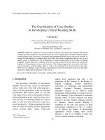
studies, at least ten additional demographic studies of Spotted Owls were initiated between 19891992. The 11 studies represented in the following
chapters occurred in most of the physiographic
provinces within the range of the owl (Figure 1).
Between 1983-1993, researchers on the various
study areas banded over 7,000 Northern Spotted
Owls. Collectively, these studies constitute the
largest detailed population dynamics study based
on mark-recapture methods of a predatory bird
ever conducted.
The Spotted Owl controversy has resulted in
a proliferation of mathematical population models designed to investigate the hypothetical responses of owl populations to different kinds of
landscape management. Lande (1987, 1988) first
explored extinction theory relative to Spotted
Owls. Noon and Biles (1990) then used models

to examine the sensitivity of the finite rate of
population change to estimated vital rates. Territory cluster models, spatially explicit population models, and dispersal models also have been
developed to explore conservation strategies for
Spotted Owls (e.g., Thomas et al. 1990, Lamberson et al. 1992, Carroll and Lamberson 1993,
McKelvey et al. 1993, Boyce et al. 1994, Raphael
et al. 1994, Bart 1995).
We emphasize that population models and
theory have been used primarily to examine hypothetical population performance under different sets of assumptions about landscapes and

OWLS-

Gut@rrez et al.

FIGURE 1. Location of known territorial Spotted
Owl pairs, singleowls, and demographicstudy areas
in the PacificNorthwest.

behavior. They cannot be regarded as definitive
analyses of population processesor performance.
Nevertheless, demographic information and
population models have become “weapons of
choice” among competing advocacy groups (see
below). The distinction between population
modeling and population analysis is blurred in
the mind of the public. The first is an abstraction
and the latter is an objective assessment of empirical data. Population models are constructed
by depicting, mathematically, the characteristics
of a population and then examining the hypothetical population behavior under a variety of

8

STUDIES

IN AVIAN

assumptions. They can be simple or complex
depending on the number of parameters used
and their purpose. Models can be constructed
without knowledge or estimates of the actual parameter values. That is, one can guess at the
value or limit of specific parameters. Therefore,
population models can be far from reality if the
parameters used to qualify the model are incorrect. On the other hand, population analyses,
such as those represented by the following chapters, are based on objective evaluation of the life
history information of the bird derived by capturing, marking, and resighting the same birds
over long periods of time. It is the latter scientific
process that currently drives inferences about the
status of the Northern Spotted Owl, and is the
subject of the chapters in this volume.
USE OF DEMOGRAPHIC
MANAGEMENT
PLANS

DATA

IN

THE 1988 FINAL ENVIRONMENTAL IMPA(TT
STATEMENTFOR THE NOR THWEST REGION
OF THE U.S. FORESTSERVICE

The first attempt to use demographic information for management was a truncated life table analysis based on preliminary estimates of
vital rates derived from mark-recapture studies
of banded owls and telemetry studies of juvenile
owls (USDA 1988). The risk of population decline was evaluated under a set of alternative
management strategies. The efficacy of the proposed management strategy (a series of widely
spaced 400-ha habitat islands managed for individual owl pairs) was considered poor based
on this analysis. Litigation (Seattle Audubon vs
Evans 1989) forced abandonment of this management strategy primarily because the demographic analysis indicated a poor long-term prognosis for the owl population.
THE INTERAGENCYScIENmK Coh%m-r~~ (ISC)
In 1989 a group of scientists was selected by
the affected Federal agencies charged with managing Spotted Owls to develop a scientifically
credible conservation plan for Northern Spotted
Owls on federal lands (Thomas et al. 1990). This
team initially addressed the problem by asking
four questions, two of which were related to demography: (1) are Spotted Owl populations declining?, and (2) are there gaps in the distribution
of owls resulting from human-caused factors?The
ISC concluded that the answer to these questions
was “yes.” The ISC proposed a conservation
strategy that included a system of relatively large
habitat conservation areas distributed across the
range of the owl. Demographic information was
used to estimate theoretically the minimum size
of reserves necessary to maintain short-term

BIOLOGY

NO. 17

(< 100 years) population stability as well as to
evaluate scenarios of range-wide distributions of

owls. Although criticized as inadequate by some
scientists and environmental groups (e.g., Harrison et al. 1993), the conservation strategy proposed by the ISC served as the model for a series
of subsequent owl and old-growth forest conservation plans. The USDA Forest Service issued
a directive to manage in a manner “not inconsistent with” the ISC plan, but litigation forced
the agency to broaden the management plan to
include all late-successional forest speciesas well
(Seattle Audubon Society vs. Mosley civil case
No. C92-479WD).
THE NORTHERN SFQTTEDOWL LISTING
DECISION
A petition to list the Northern Spotted Owl
under the Endangered Species Act was filed with
the U.S. Fish and Wildlife Service in 1987. The
U.S. Fish and Wildlife Service completed a status
review in December 1987 and concluded that
listing was not warranted. This decision was
challenged in U.S. District Court in 1988 (Northem Spotted Owl and Seattle Audubon Society
vs. Hodel, civil case No. C88-5732). The court
ruled that the decision to not list the owl was
arbitrary and capricious, and instructed the Service to reexamine the issue (see GAO 1989 for
a review). Following a review of the evidence by
another status review team and a listing review
team (Anderson et al. 1990), the Northern Spotted Owl was listed as “threatened” in 1990 (USDI
1990). Habitat loss, apparent population declines, and failure of existing regulatory mechanisms to protect the owl were the primary reasons cited for listing. Information gathered from
demographic studies was used extensively by the
teams to evaluate the population status of the
owl.
SCIENTIFIC PANEL ON LATE-SUCCESSIONAL
FORESTE~GSYSTEMSREPORT TO THE
U.S. HOUSE OF REPRE~ENTA-~IVE~

In 1991, following a request from two committees in the House of Representatives, a team
of four scientists was formed to develop a series
of alternative strategies for the management of
mature and old-growth forests in the Pacific
Northwest (Johnson et al. 199 1). This team developed 14 different alternatives for the management of old forests, 12 of which were based
on a network of large reserves similar to the reserve design proposed by the ISC for Spotted
Owls. The size and spacing of the proposed reserves were heavily influenced by the analyses of
owl demography conducted by the ISC, and by
consideration for Marbled Murrelets (Bruchyramphus marmoratum) and fish. None of the op-


DEMOGRAPHIC

STUDIES

OF SPOTTED

tions proposed by the panel was ever officially
adopted. However, these options played a major
role in subsequent plans for owls and old forests.
THE NORTHERN SPOTTEDOWL RECOVERYPLAN
A Northern Spotted Owl recovery team was
formed in 1990. The team was unique among
recovery teams because it was appointed by the
Secretary of Interior and the majority of the team
members were non-scientists (Gutitrrez 1994b).
The recovery team used the ISC reserve design
as a working model for the design proposed in
the recovery plan. However, the recovery team
departed from the standard format of identifying

numerical targets as de-listing criteria. Rather,
the de-listing criteria were based on trends in
demographic rates within specific physiographic
provinces (USDI 1992b). In other words, population processes were emphasized rather than
simple numbers. This departure from tradition
was necessary because (1) Spotted Owls were still
relatively numerous in most provinces, (2) census information was incomplete, and likely to
remain so, (3) logging was still allowed under the
plan, and (4) the existing demography studies
demonstrated that owl trends could be monitored.
Anderson and Bumham (1992) analyzed the
extant demographic data for the recovery team.
Their results indicated that Spotted Owl adult
female mortality was accelerating over the period
during which the demography studies occurred.
This result directly led a Federal Court judge to
reject the 1992 U.S. Forest Service Spotted Owl
EIS.
The Recovery Plan, like the ISC plan, assumed
that owl populations would reach a new lower
carrying capacity where they would eventually
stabilize. Thus, it was likely that owl numbers
would continue to decline in the near term or
until habitat recovery within designated conservation areas balanced loss of habitat outside of
conservation areas. The recovery plan was completed in 1992 but was never formally released
by the USDI.
THE ENDANGEREDSPECIESCOMMITTEE
During the recovery planning process, the Director of the Bureau of Land Management (BLM)
requested that a cabinet-level committee be convened to determine the fate of 44 proposed timber sales on BLM lands in western Oregon that
had been found by the U.S. Fish and Wildlife

Service to “jeopardize” the Northern Spotted
Owl. After an evidentiary hearing in January 1992
before an administrative law judge, the committee acted to protect all but 13 of the sales
from logging. The primary reasons for the continued protection was the potential negative de-

OWLS-

Guti&rez

et al.

9

mographic consequences to the owl population.
Of particular concern was the potential loss of
habitat connectivity between physiographic
provinces. The demographic information derived from the population studies was key to the
discussion of possible demographic consequences of the proposed logging. The 13 sales
were subsequently withdrawn from logging by
the BLM.
THE SCIENTIFIC ANALYSIS TEAM (SAT)
In response to instructions from a federal court
judge, the Chief of the Forest Service convened
a panel of scientists to assessthe viability of species associated with old forests on Forest Service
lands within the range of the Northern Spotted
Owl. This was the first time that the Forest Service had formally attempted to evaluate proposed plans for the Spotted Owl in a broader
ecosystem context. After examining the demographic data on the Spotted Owl, the SAT concluded that I‘. . . demographic rates or trends observed during a prolonged period of habitat loss
will provide little insight as to whether the population will eventually reach a new stable equilibrium when the rate of habitat loss is equaled
by the rate of habitat gain . . .” (Thomas et al.
1993a: 192). This opinion was in stark contrast

to the opinions of some other scientists and environmental advocates who had suggested that
the negative trends in demographic data were
evidence that proposed agency plans for the owl
were inadequate (e.g., Harrison et al. 1993).
THE FORESTECOSYSTEMMANAGEMENT
TEAM (FEMAT)

ASSESSMENT

In 1993, the Clinton Administration initiated
an effort to resolve the Spotted Owl/old-growth
forest impasse by appointing a team of scientists
to develop a comprehensive plan for the management of late successional forests on federal
lands in the Pacific Northwest (Thomas et al.
1993b). The ten management options proposed
by the FEMAT included provisions for various
levels of protection for Spotted Owls as well as
other late seral stage forest species. The option
selected by the Administration (referred to as
“Option 9”) was similar to several previous plans
(Thomas et al. 1990, Johnson et al. 199 1, USDI
1992b), with some modifications in reserve design and major changes in recommendations for
management of forest lands between the reserve
network. Although FEMAT
discussed demographic data from capture-recapture studies in
their analysis, they concluded that current demographic data alone were not appropriate to
assessthe outcome of a management plan that
would not produce the desired mix of habitats
until approximately 100 years after implemen-

10

STUDIES

IN AVIAN

tation. After release of the FEMAT report, some
scientists and environmental activists suggested
that the negative trends in population parameters
reported by Anderson and Bumham (1992) were
sufficient to warrant an immediate cessation of
all logging of owl habitat (e.g., Harrison et al.
1993). This view was supported by a group of
14 scientists who wrote a letter to the Secretaries
of Interior and Agriculture in September 1993,
requesting that implementation of Option 9 be
delayed until a full review of all existing demographic information on the Northern Spotted Owl
was conducted.

THE 1993 FORTCOLLINS WORKSHOP
Several industry groups and timber companies
began population studies of Spotted Owls in
1990-l 99 1. These studies paralleled other studies on Federal lands, and resulted in relatively
large numbers of owls being located and banded
in young and mid-aged (40-70 years) forests in
some areas (most notably northwestern California and the east slope of the Cascades in Washington). These findings were interpreted by some
as an indication that Spotted Owls were thriving
in young forests (e.g., Easterbrook 1994), and
motivated a de-listing petition for Spotted Owls

in California (California Forestry Association
1993). As a result of this de-listing petition and
the previously mentioned September 1993 letter
from a group of concerned scientists, the Secretaries of Interior and Agriculture requested in
October 1993 that a workshop be immediately
convened to update and analyze all demographic
data on the Northern Spotted Owl.
All researchers having three or more years of
demographic information were invited to attend.
Eleven research groups participated. One industry group participated initially, but withdrew their
results before the end of the workshop. Two other
invited industry groups did not present their data
for analysis. The results of the analyses conducted at Fort Collins were provided to the U.S.
Forest Service and Bureau of Land Management
for inclusion in their planning documents. The
results of the individual study area analyses and
the meta-analysis of the entire data set form the
basis for the individual chapters that follow this
review.
THE 1994 U.S. FORESTSERVICEAND BLM
FINAL SUPPLEMENTALENVIRONMENTAL
IMPACT STATEMENT(FEIS)
In February 1994, the USDA Forest Service,
USDI Bureau of Land Management, and several
other federal agencies released a joint FEIS for
the management of late successionalforests within the range of the Northern Spotted Owl (USDA
and USDI 1994a). A formal presentation of the

BIOLOGY

NO. 17

summary data from the Fort Collins demographic workshop was included in the FEIS (Bumham
et al. 1994b). The Record of Decision for the
FEIS (USDA and USDI 1994b) was to proceed
with implementation of Option 9 (now Alternative 9) on Federal lands, with some adjustments to improve dispersal habitat and to protect
additional pairs of owls in some provinces. Despite the negative population trends estimated
from the demographic data examined at Fort
Collins, it was the opinion of the FEIS Team that
the owl population would likely reach equilibrium once the habitat conditions specified in Alternative 9 were attained. A spatially explicit
population model (McKelvey et al. 1993), parameterized with demographic data, was used to
evaluate the performance of the preferred alternative assuming a range of birth and death rates.
ADVERSARIALPROCEEDINGS
Demographic information and estimates of
habitat loss have been central to litigation and
procedural arguments levied by competing advocacy groups (i.e., environmental and industry
groups). Demographic trends have been a critical
element in this process. Some scientists and environmental activists have relied on demographic trend information and estimates of vital rates
derived from demographic studies to suggestthat
proposed plans do not adequately protect the
Spotted Owl (e.g., Harrison et al. 1993, Lande et
al. 1994). Other scientists and industry advocates
have countered by suggesting that the demographic data may be flawed or that models used
to analyze the data may be overly simplistic or
inappropriate (e.g., Boyce 1987, Boyce et al. 1994,
Bart 1995). In addition, some have tended to
emphasize the results of models on demographic
processes(e.g., Lande et al. 1994), whereas other
groups have emphasized the relatively large size
of the owl population (e.g., California Forestry

Association 1993). Some scientists associated
with the demographic studies of Spotted Owls
have assumed a more cautious position, suggesting that there is uncertainty regarding interpretation of the data, and that all of the protagonists should avoid extreme positions (e.g., Thomas et al. 1993a, USDA and USDI 1994a).
SUMMARY
Management of the Northern Spotted Owl is
an extremely contentious conservation issue involving many interest groups with divergent
views about how the needs of the owl and society
should be balanced. It has become a biopolitical
cornerstone of large scale conservation policy.
Wildlife scientists have played a key role in the
development of conservation strategies for the


DEMOGRAPHIC

STUDIES

OF SPOTTED

owl and have made extensive use of empirical
data from mark-recapture studies for assessing
trends in vital rates and for parameterizing theoretical population models. Demographic information, gathered from a series of studies across
the range of the owl represents the most detailed
population dynamics study of a predatory bird
ever undertaken. This information has been used
in unique ways and has strongly influenced the
conservation ofthe owl and its habitat. The Spotted Owl issue is unique among endangered species problems because owls were widespread and
relatively common over much of their range when
demographic studies began. The assessment of
birth and death rates to estimate population

trends was necessary because estimating changes
in owl habitat, or in overall numbers of owls,
were insufficient tools to adequately assesspopulation trends. In essence, biologists were asked
not only to estimate the status of different owl
populations but also to estimate how much logging could continue while local populations declined. Because the owl primarily inhabits oldgrowth and mature forests on public lands, declining populations have resulted in substantial
restrictions in logging on public lands. Decisions
to restrict harvest have been considerably influ-

OWLS-

Gutihez

et al.

11

enced by demographic studies of Spotted Owls
conducted between 1985-1993. We present a
brief history of the role of demographic data in
the development of management strategies for
the owl.
In addition to the utility of demographic information for the solution of a resource problem,
these studies have stimulated theoretical work in
such areas as extinction thresholds, population
dynamics, dispersal, and reserve design (Lande
1987, 1988; Doak 1989; Thomas et al. 1990;
Franklin 1992; Lamberson et al. 1992, 1994).
Thus, the demographic studies in the following
chapters serve as an example of the effectiveness
of coordinated research to problem solving and

the advancement of science.
ACKNOWLEDGMENTS
We thank D. Kristan, L. Brennan, C. de Sobrino,
M. Raphael, S. DeStefano, and two anonymous reviewers for their comments on the manuscript. Financial supportwasprovided by the USDA Forest Service,
USDI Fish and Wildlife Service,USDI Bureauof Land
Management, State of California ResourcesAgency,
California Department of Fish and Game, Oregon Department of Fish and Wildlife, and Washington Department of Wildlife and Fish.

Key words: conservation strategies, demography, Northern Spotted Owl, Strix occidentalis caurina.


Studies in Avian Biology No. 17: 12-20, 1996.

METHODS FOR COLLECTING
AND ANALYZING
DEMOGRAPHIC
DATA ON THE NORTHERN
SPOTTED

OWL

ALAN B. FRANKLIN,DAVID R. ANDERSON,ERIC D. FORSMAN,
KENNETHP.BURNHAM,ANDFRANKW.WAGNER
INTRODUCTION

studies on the Northern Spotted Owl, we feel this
paper will also provide a framework useful for
similar research with other raptors. Terminology
and symbols used throughout this volume are
presented in the Appendix.

The collection of demographic data reflecting
birth and death rates is important for understanding the life-history characteristics and population trends ofthe Northern Spotted Owl (Strix
occidentaliscaurina). Demographic parameters
generally take the form of age-, sex-, and timespecific survival probabilities and fecundity rates.
The first step in assessing the validity of inferences derived from such data is demonstration
of an appropriate study design, as well as the
field and analytical methods used. In addition,
the methods used to collect demographic data
should be repeatable, logistically feasible, and
support the internal validity of the study design.
Both study design and methods used to collect
demographic data in the field must support the
assumptions of models used to analyze those data
for valid inferences to be made.
Demographic studies of Northern Spotted Owls
reported in this volume are unique in several
ways. First, these studies have been able to incorporate capture-recapture modeling approaches to estimate survival probabilities. These types
of models have been rarely used with raptors,
primarily because of sample size limitations (see
Blonde1 et al. 1990 for reviews on different avian
taxa). Second, standardized methods have been
incorporated across all studies reported in this
volume. This allowed for consistency in data collection and, hence, consistency in interpretation
of results across the range of the owl. Third, the
spatial extent and spatial replication of demographic studies allowed for broader inferences
across the species’ range in a meta-analysis (see
Bumham et al. this volume).
The purpose of this paper is to present common elements of field and analytical methods
used to estimate demographic parameters and

population trends in Northern Spotted Owls as
reported in this volume. We provide general descriptions of study areas, methods of data collection, and analytical methods used to estimate
demographic parameters. Specific methods used
in individual studies which depart from this general overview are described in the specific chapters pertaining to those studies. We also address
important assumptions pertinent to the analytical models used and the allowable scope of inferences. Although confined to demographic

STUDY

AREAS

This volume includes data from 11 study areas
in northern California, Oregon and Washington
(Fig. 1). Combined area of these study areas was
45,846 km2 (Table 1). All of the study areas were
primarily located on public lands administered
by the U. S. Forest Service, U. S. Bureau of Land
Management, and National Park Service. Inclusion of privately-owned lands in most study areas occurred incidentally as “inholdings” within
public lands. However, most study areas on Bureau of Land Management districts included
nearly equal mixtures of federal and non-federal
lands. Inferences concerning Spotted Owl populations were restricted primarily to federally administered lands within the range of the owl except for the Bureau of Land Management studies
(Coos Bay, Eugene BLM, Salem BLM, Roseburg
BLM, and South CascadesSiskiyou; see Fig. 1)
which contained large amounts of private land.
The 11 study areas encompassed about 27% of
the 98,967 km2 of federally administered land
within the range of the Northern Spotted Owl
and about 20% of the 230,690 km* range of the
Northern Spotted Owl (USDA and USDI 1994).
Study area selection in all the owl demographic
studies was based primarily on logistic considerations and objectives of funding agencies. As

a result, study areas were not randomly or systematically distributed across the geographic
range of the owl. Most studies were concentrated
in the coastal mountains of California, Oregon,
and Washington with fewer studies in the Cascade Mountains. We do not know if this uneven
distribution of study areas caused bias in the
overall evaluation of Spotted Owl populations
across their range. However, the overall opinion
of the research biologists at the Fort Collins
workshop (see Gutierrez et al. this volume) was
that the broad representation of study areas from
different forest types and management regimes
was probably reflective of the overall condition
of Spotted Owl populations on federal lands.
12


DEMOGRAPHIC

METHODS

FOR

SPOTTED

Of the 11 study areas, eight included intensively surveyed areas referred to as Density Study
Areas (DSAs) (Table 1). DSAs were 204-1011
km* in size and established a priori with boundaries based on major topographical features and
ownership boundaries. All habitats within DSAs
were intensively surveyed for Northern Spotted
Owls each year (Franklin et al. 1990), including

at least two replicate surveys of each area each
year. Minimum size for DSAs was established
based on criteria outlined in Franklin et al. (1990)
to minimize bias in density estimates due to edge
effects. Maximum size for DSAs was dictated by
the investigator’s ability to survey adequately the
entire area given funding and logistical constraints. Outside of the DSAs, no attempt was
made to survey entire study areas each year.
Rather, surveys focused on specific sites that had
a history of occupancy by Spotted Owls. A “site”
was defined as an area where Spotted Owls had
exhibited territorial behavior in response to surveys on two or more occasions separated by one
or more weeks within a given year. Individual
sites were surveyed each year regardless of
whether they were occupied by Spotted Owls.
The use of the two types of survey design (DSAs
versus site-specific surveys) reflected a trade-off
between gathering additional information on
movements and density in the DSAs and increasing sample size and regional scope in the
larger study areas.
Two important assumptions regarding study
area selection are: (1) study areas are representative of the larger area to which inferences are
made, and (2) banded owls within a study area
are representative of the population within that
area. Whereas the first assumption can be objectively examined by comparison of landscape
composition within and outside study area
boundaries, the second assumption can not be

TABLE

1.

Dmcxmrt

ONOFTHE

OLY
CLE
SAL
SIU
HJA
EUG

OWLS-Frankfin

Olympic Peninsula
Cle Elum
Salem BLM
Siuslaw NF
H.J. Andre’.%
Eugene BLM

coo
RSB
SCS
SIS
CAL

et al.

13

coos Bay BLM
Roseburg BLM
S. Caxades/Slskiyou
Siskiyou
NW California (Wiilow Creek)

FIGURE
1. Location of 11 study areas used to estimate demographiccharacteristicsof Northern Spotted Owls.

~~DEMOGRAPHIC STLJDYAREAS~RTHENORTHERNS~TEDO~L

Study area @cation)

Willow Creek (NW California)

ACKlOpl

Roseburg (Oregon)

CAL
RSB

S. Cascades & Siskiyou Mts. (Oregon)

scs

Salem BLM (Oregon)
H. J. Andrews (Oregon)

Olympic Peninsula (Washington)
Cle Elum (Washington)
Eugene BLM (Oregon)
Coos Bay (Oregon)
Siuslaw NF (Oregon)
Siskiyou NF (Oregon)

SAL
HJA
OLY
CLE
EUG
coo
SIU
SIS

Study area

size(kn?)
1,784
6,044
15,216

3,249
1,075
8,145
1,763
2,082
2,477
2,749

1,262

DSA
size(km')
292
310
326
1,011
300
491
300
355
196
273
676
-

Yeamofbanding
1985-1993
1985-1993
1985-1993

1986-1993
1987-1993
1987-1993
1989-1993
1989-1993
1990-1993
1990-1993
1990-1993

14

STUDIES

IN AVIAN

tested. However, there are three lines of evidence
which suggest that assumptions 1 and 2 were
probably met. First, the 11 demographic studies
encompassed over a quarter of the federal lands
within the geographic range of the owl and were
reasonably well-spaced throughout that range.
This suggests that a large portion of the variability present within the owl’s range was probably captured. Second, 3,6 16 territorial individuals (exclusive of 2,443 juveniles) were marked
during these studies (Burnham et al. this volume)
out of a known population of about 6,000 territorial individuals on federal lands in Washington, Oregon, and California (U.S. Dept. Interior
1992). While not all of these marked individuals
were alive at the same time, a large portion of
the range-wide population was probably marked,
especially considering the high survival rates for
PZ l-year old owls (Bumham et al. this volume).
Third, all research biologists, whose study areas
are represented in this volume, agreed that their
study areas were not grossly different from habitat amounts and configurations in the matrix
surrounding their study areas.
METHODS
FIELD METHODS
The general design of the demographic studies,
described in the following chapters, consisted of

tracking marked individuals and their associated
life history traits over time. Each study area was
annually surveyed to locate both marked and
unmarked owls. Once owls were located, they
were individually marked using unique color
bands and numbered U. S. Fish and Wildlife
Service (USFWS) bands. Age, sex, and reproductive status of individuals were determined
with standardized techniques as detailed below.
Thus, for each year, individuals were located,
assigned an age-class, identified, and assigned an
estimate of their reproductive output.

Surveys
Annual surveys for Spotted Owls were conducted between 1 March and 1 September. Spotted Owls were located using vocal imitations or
recorded playback of their calls to elicit responses
(Forsman 1983). Both day and night surveys were
used to locate owls (Forsman 1983). The primary
method for surveying at night was calling for
2 10 min from a series of stations spaced 0.30.5 km along forest roads or trails. “Leapfrog”
surveys were also used where two observers alternated walking along continuous transects. Owls
were visually located by conducting calling surveys during the day to identify them and determine their reproductive status. Daytime surveys
usually focused on areas where owls had previ-

BIOLOGY

NO. 17

ously responded during nighttime surveys or
where owls had been located in previous years.
Most daytime surveys were conducted while hiking cross-country.

Survey effort generally increased in the first
few years of each study after which it leveled off.
A site was assumed unoccupied if Spotted Owls
were not detected after 3-6 night surveys, spaced
24 days apart, that completely covered 4-l 6 km2
around locations where owls had been previously
located during the day. In areas outside of DSAs,
the area searched for owls depended on locations
of adjacent pairs of owls and topography. Individuals were considered territorial if they exhibited vocal responses to surveys within the same
site on ~2 separate occasions within the same
sampling period.

Determination of sex and age
With the exception ofjuveniles, the sex of owls
> 1 year old was distinguished by calls and behavior. Males emit lower-pitched calls than females and do not incubate or brood (Forsman
et al. 1984). Juveniles could not be accurately
sexed until 1992 when some researchers began
determining sexes of juveniles through examination of sex chromosomes in blood samples
(Dvorak et al. 1992; see chapters on individual
studies).
Spotted owls were aged by plumage characteristics (Forsman 198 1, Moen et al. 199 1) either
visually, using binoculars, or when captured. Four
age-classeswere used:juvenile (J), 1-year old (S l),
2-year old (S2), and 23-years old (A). Juveniles
were fledged young-of-the-year that were characterized by gray, downy body plumage and retrices with triangular, tufted, white tips through
their first summer. One-year old birds possess
basic body plumage but are distinguished by tufted white tips on their retrices. Two-year old birds
lose the tufts on the tips of the retrices but retain
the triangular white tips until the retrices are first
molted during the third summer of life. Thereafter, they become indistinguishable from 13year old owls that have retrices with rounded

and mottled tips.

Capture and marking
Individuals were identified by initial capture,
marking, and subsequent recapture or resighting
of colored leg bands. Owls were captured with
noose poles (Forsman 1983), snare poles, baited
mist nets, or by hand. Handling time of captured
owls was typically less than 20 minutes. Each
owl was marked with a USFWS 7B numbered
lock-on aluminum band placed on the tarsometatarsus. A colored plastic leg band placed on
the opposing tarso-metatarsus was used to identify 2 1-year old birds in subsequent years with-


DEMOGRAPHIC

METHODS

FOR SPOTTED

out recapture. Some researchers modified the
color-band by adding a colored vinyl tab to increase the number of color combinations. Protocols for resighting color-marked individuals
generally included blind trials where records of
color combinations of owls located at a site in
previous years were not examined until after a
survey for that site was completed. If identification of color-marks was ambiguous, birds were
recaptured and the number from the USFWS
band recorded. Juveniles were marked with
striped color bands indicating the year when they
were captured. Cohort bands were replaced with

unique color combinations when juveniles were
recaptured in later years. The use of both USFWS
and color bands allowed us to evaluate band loss.
Only two cases of band loss were confirmed in
over 6,000 marked individuals indicating the rate
ofband loss was very nearly zero. In some studies
(see Forsman et al. this volume, Reid et al. this
volume, and Wagner et al. this volume), radiotransmitters were used on a portion of the birds
captured.

Estimation of reproductiveoutput
We used field estimates of reproductive output
(the number of young leaving the nest [fledging]
per territorial female) as the basis for estimating
fecundity. The average date of fledging (1 June)
was considered the birth date. Once located during the day, owls were checked for reproductive
activity by feeding them live mice (a procedure
referred to as mousing) and observing how they
behaved after mice were taken (Forsman 1983).
Breeding Spotted Owls usually took such offered
prey and carried it to the nest or fledged young.
Non-reproductive owls either ate or cached the
mice. Non-reproduction was inferred if an individual took ~2 offered mice, and cached the
last mouse taken, or a female did not have a welldeveloped brood patch during April+arly May
(the normal incubation period). In some cases,
we also examined brood patches during the incubation period to determine if females were
nesting. Territorial individuals were visited at
least twice during the sampling period to determine the number of fledged young or to confirm
non-reproduction using either the mousing or
brood patch criteria on each visit. These techniques enabled us to characterize the reproductive output of territorial individuals as having 0,

1, 2, or 3 fledged young.
ANALYTICAL METHODS

Estimation of survival
Capture-recapture models were used to estimate age- and sex-specific survival for Northern
Spotted Owls from the banding data. These models were statistical constructs used to estimate

OWLS-Franklin

et al.

15

the parameters ofinterest from the empirical data.
The statistical analysis of capture-recapture or
resight sampling data was based on the theory
derived by Cormack (1964) Jolly (1965) and
Seber (1965) and the simplifications and generalizations published since that time (e.g., Burnham et al. 1987, Clobert et al. 1987, Pollock et
al. 1990). Lebreton et al. (1992) provided a comprehensive review of these theories, with examples. The capture history (Bumham et al. 1987:
28) for each owl for each age and sex class provided the basis for parameter estimation and hypothesis testing. The capture history matrix (X,
described below in Parameterization) is a complete summary of the data. Estimators for all
models used various summary statisticsfrom this
matrix. Owls were not included in the analysis
during the time they carried back-pack transmitters because these types of transmitters may
affect survival (Paton et al. 199 1, Foster et al.
1992). However, owls fitted with 5-gram tailmounted transmitters (mostly juveniles) on three
study areas were included in the capture-recapture analyses because there was no evidence such
small transmitters affected survival (E. Forsman,
unpublished data). Owls with tail-mounted
transmitters were considered recaptured only if

they were located and their identity confirmed
during normal calling surveys without the use of
radio-telemetry. This ensured that recapture
probabilities were not biased by differential detection of radio-marked birds. We assumed a 1: 1
sex ratio at fledging for years where juveniles
were not sexed. For each cohort of banded juveniles, the individuals subsequently recaptured
were sexed and the remaining capture histories
(representing individuals never captured) were
arbitrarily assigned as males or females such that
the total number of males and females was equal
(Franklin 1992). The assumption of a 1: 1 sex
ratio was supported by data on juveniles sexed
using chromosomal analysis (see Franklin et al.

this volume).
Parameterization. The basic model for open
mark-recapture populations is the Cormack-Jolly-Seber (CJS) model (Cormack 1964, Jolly 1965,
Seber 1965) which considers only time specific
survival probabilities (+i) and recapture probabilities Q_+)for k capture occasions (see Appendix
for full summary of notation). These parameters
are conditional on an animal being alive at the
beginning of occasion i. Survival probabilities
are estimated between occasion i and i+ 1 where
i= 1,2
. . 2k - 1. Recapture probabilities are
the probability that an animal alive on occasion
i is captured (or recaptured) where i = 2, 3, . . . , k
(p, is not defined). In the case of the Spotted Owl,
“capture” is defined as physical capture of individuals or resighting of their color bands with-

STUDIES

16

IN AVIAN

out physical capture. The pi are nuisance parameters, but must be properly treated or estimators
of survival probabilities will be biased. For example, let @i be the survival probability between
sampling occasions 1 and 2 and&be the survival
probability between occasions 2 and 3. Therefore, for k = 3 capture occasions, the probability
of various capture histories can be parameterized
as: Pr{ lOl} = 4,q2&p3 (where q, = 1 - pi, the
probability of not being captured on occasion i)
for individuals captured on the first and third,
but not the second, occasion; Pr{ 1 1 1 } = &p2&p3,
for individuals captured on all three occasions;
and Pr{ 1 lo} = &p2&q3, for individuals captured
on the first and second, but not the third, occasion. Assuming the fates of individual animals
were independent and that they have the same
parameters (I#J~
andp,), the data on first recaptures
from a single released cohort has a multinomial
distribution. Releases from several cohorts are
merely a product of these multinomial distributions. The likelihood function follows from
this expression and is the basis for statistical inference.
Parameter estimation was based on Fisher’s
method of maximum likelihood. This method
provided estimators of parameters that were asymptotically unbiased, efficient, and normally
distributed. Variances and covariances were estimated using quasi-likelihood methods where

appropriate (Wedderbum 1974, Cox 1983). These
methods allow year- and age-dependent variation to be included in the variance of estimators
from models that assume parameters were constant over years or age classes.For example, with
the CJS model for a 3-occasion survey, four possible fates were possible for owls marked and
released at occasion 1: X, , , , X, ,0, X,,,, and Xi,, .
Then the likelihood function of the unknown
parameters, given the data (X) will be:
L&i, Pi I Xl

(41w#JzP3)x’y( 1 -f#&*(

1 -d&$QOO

where C is the multinomial coefficient, involving
the data, but not the parameters.
The analysis of multiple data sets provided
extensive model building opportunities beyond
the CJS model (Lebreton et al. 1992). Relationships of rates to external variables were modeled
in this framework using the logit(0) transformation which constrains 0 5 0 5 1 as
logit(0) = In &
(

)

where 6’represents either $ or p. Lebreton et al.
(1992) and Hosmer and Lemeshow (1989) pre-

BIOLOGY

NO. 17

sented rationales for use of this logit-link function. Survival probability (4) and recapture probability (p) could then be modeled as a linear
logistic function,
logit (0,) = PO + P,(w)
where w is an external or dummy variable. This
approach allowed both categorical (e.g., sex,
groups) and continuous (e.g., linear time) covariates to be employed in modeling 4 or p. Lebreton et al. (1992) provided examples of these
approaches and more extended theory. We used
programs RELEASE (Bumham et al. 1987) and
SURGE (Pradel et al. 1990) for analysis of markrecapture data.
An important consideration with survival
probabilities derived from capture-recapture estimators is that 1 - 4 = (mortality rate + permanent emigration rate) whereas with true survival (S), 1 - S = mortality rate only. In order
for 4 = S, permanent_ emigration (E) must be
negligible. Therefore, 4 must be adjusted when
E is substantial to reflect true survival probabilities. Some studies ( see Bumham et al. this
volume, Forsman et al. this volume, Reid et al.
this volume, and Wagner et al. this volume) used
data from radiomarked owls to adjust some estimates of 4 for E (seeBumham et al. this volume
for methodology).
Model notation. Model nomenclature (see Appendix) followed Lebreton et al. (1992) and can
be summarized as follows. The basic CJS model
has time-specificity only, which can be expressed
as {&, p,}. This notation indicates a model whose
parameters have unrestricted variation solely over
time (occasions). If sex (s) or group (g, e.g., where
g = study area) effects are added to the model,
it can be written as {A.,, p,.,} where parameters
exhibit unrestricted variation in time within each
sex class, or {e&, p,.,} where there is a group
effect other than sex. The asterisk (*) indicates

interactions (e.g., s* t indicates interactions of sex
with time, as well as both main effects). Therefore, a model examining study area effects, sex
effects and unrestricted time variation for 1 ageclass would be denoted as {&.s.t, p,.,.,}. Age (a)
can also be added as a factor and combined with
sex, time and group effects in the same manner.
The pure age model is denoted as {4,, pa} where
parameters vary by age only and, for k occasions,
a= 1,2,...,
k - 1 ages. Models that include
age restricted to classes are denoted as a 1, a2,
a3,. . . , an where n is the number of age-classes
used. In models where pi were age-specific for
birds initially banded as juveniles, parameters
are subscripted as an’ where n’ is the number of
age-classes over which the restrictions are applied. Additive effects (i.e., no interactions considered) in models are denoted with a +
‘ ’ instead


DEMOGRAPHIC

METHODS

FOR SPOTTED

ofa *‘.‘ For example, the subscript s + t indicates
that the subscripted parameter varies over time
for both sexesbut that the difference between the
two sexes is constant over time; plots of logit
parameter estimates over time for the two sexes
would be parallel. Parameters also can be constrained as linear functions of time, denoted as

T. The resulting models are similar to the classical analysis of covariance where (1) parameters
subscripted as T represents one intercept and one
slope estimated for the parameter over time [logit(d,) = /3,,+ p1 (time effects)]; (2) s + Trepresents
different intercepts for each sex with a common
slope [logit
= /I0 + /3, (sex effects) + & (time
effects)]; and (3) s* T represents different intercepts and slopes for each sex [logit(4i) = ,& + 0,
(sex effects) + & (time effects) +& (sex effects *
time effects)]. The H,: p = 0 for estimated slope
parameters is tested using a Wald test (Carroll
and Ruppert 1988, Hosmer and Lemeshow 1989)
of the form:
-2
X2 = - P

with 1 df

v%r@)

Tests of assumptions. Goodness of fit tests
(Pollock et al. 1985, Burnham et al. 1987) were
used to assess the adequacy and utility of the
basic CJS model, {$J,,p,}. Burnham et al. (1987)
outlined the requisite assumptions as: (1) capture, handling, and release do not affect survival;
(2) the number released on occasion i is known
exactly; (3) there is no band loss, and no bands
are misread on capture or resighting; (4) all releases and captures of owls occur in relatively
brief time intervals, and recaptured birds are released immediately; (5) any unknown emigration
out of a study area is permanent (e.g., owls do
not become unavailable for recapture by temporarily leaving the study area); (6) the fate of

each individual owl, after any known release, is
independent of the fate of any other owl; (7) data
sets for the various ages, sexes, and areas are
statistically independent; (8) statistical analyses
of the sample data are based on an appropriate
model; and (9) all owls of an identifiable class
(e.g., age, sex) have the same survival and capture
probabilities, by study area (i.e., parameters are
homogenous within subclasses of individuals).
Assumption (1) was tested using TEST 3 of program RELEASE which tests whether previously
released individuals have the same future fates
as newly released individuals. Assumption (2)
and (3) probably were met with the Northern
Spotted Owl data (see Capture and marking section). Assumption (4) was not strictly met in that
the sampling period was relatively long (3-4
months). However, di is unbiased given that the
shape of the temporal distribution of releases

OWLS-Franklin

et al.

17

(TDR) is constant from year to year and bias in
di is negligible when the medians of TDR are
equal even though the distribution shapes may
vary (inferred from Smith and Anderson 1987).
This can be tested with Kruskal-Wallis tests (Sokal and Rohlf 1981) and multi-response permutation procedures (Mielke et al. 198 1). Assumption (5) was untestable although it can be
evaluated qualitatively. We tested assumptions

(6), (7) and (9) using TEST 2 and 3 in program
RELEASE (Bumham et al. 1987). TEST 3 is sensitive to heterogeneity in $i and pi (assumption
9) short-term marking effects (e.g., assumption
l), and failure of assumption (6). TEST 2 also
tests assumptions (6) and (1) as well as assumption (7) and for temporary emigration where an
individual leaves the study area for at least one
year and then returns. Assumption (8) can be
properly evaluated through appropriate statistical model selection criteria and procedures, as
described below.
Model selection.The most critical problem in
the comprehensive analysis of capture-recapture
data involving several year, age, and sex classes
is selecting an appropriate model to describe the
data (Bumham and Anderson 1992, Bumham et
al. 1995a). A model should have sufficient structure and parameters to account for significant
variability in the data or the resulting estimates
will likely be biased. However, if the model has
too much structure or too many parameters, then
precision is lost unnecessarily. Proper model selection seeks a model that is fully supported by
the particular data set and, thus, has enough parameters to avoid bias but not so many that precision is lost (Principle of Parsimony; see Bumham and Anderson 1992).
Model building started with a global model of
i&*,.0 p,.,.,} for each study area (i.e., separate
{&,, p,,,} for each sex). We then used Akaike’s
Information Criterion, AIC (Akaike 1973, Anderson et al. 1994, Bumham et al. 1994, 1995a,
1995b), to objectively selectan appropriate “best”
model. This criterion was defined as
AIC = -2ln(L)

+ 2K

where In(L) is the natural logarithm of the likelihood function evaluated at the maximum likelihood estimates and K is the number of estimable parameters from that model. After selection of the best model using AIC, neighboring
models of interest can be further investigated
using likelihood ratio tests (McCullagh and Nelder 1983) as a further aid in selecting the best
model for a particular data set. This procedure
tests which of two nested model is best supported
by the data using Ho: the model with fewer parameters versus H,: the model with more pa-


18

STUDIES

IN AVIAN

rameters. For example, a significant P-value resulting from a test of Ho: model {&} versus H,:
{+,} indicates that {&} should be retained as the
best model, whereas a non-significant P-value
would support retention of {&}. In the same
manner, likelihood ratio tests can be used to test
for specific effects, such as sex, time, and age,
using identical models except that one includes
the effect of interest and the other does not.

Estimation of fecundity
Age-specific fecundity (b,) was defined for
Northern Spotted Owls as the average number
of female fledglings produced by a territorial female of age x (Caughley 1977). Age-specific fecundity was estimated using analysis of variance
(ANOVA). Despite the integer nature of the individual data, sample sizes were sufficiently large
to justify the assumptions of ANOVA.
Data

analysis was performed on reproductive output
as the response variable using the general linear
models (GLM) procedure in SAS (SAS Institute
1990) to test for significant age and time effects
and interactions between effectswithin each study
area. After analyses were performed, age-specific
fecundity estimates (b,) were calculated from estimates of mean reproductive output in each ageclass by dividing those estimates by 2 to account
for an assumed 1: 1 sex ratio. In keeping with the
1: 1 sex ratio assumption, standard errors of estimates for mean number of young fledged were
divided by 2 (Goodman 1960) to estimate sE(b,).
In counting number of fledged young, we assumed that detection probabilities (analogous to
p,) of broods, and individual young within broods,
after two visits was equal to 1.O. Three additional
factors may introduce bias into estimates of fecundity. First, reproductively active individuals
may have higher detectability than non-reproductively active individuals (e.g., Lundberg 1980).
Therefore, fecundity would be biased high because fewer observations of 0 young would be
recorded. Second, some fledged young experience mortality after fledging and before some
pairs are checked for reproductive activity. In
this case, the number of fledged young would be
underestimated and, hence, biased downward.
Third, some young are not banded immediately
after they are counted. This would introduce a
positive bias in the recruitment of first-year birds
into the population (b&J because fledglings that
die between the time they are counted and when
the site is revisited again to band young are not
included in the releases from which juvenile survival is estimated. It is unknown to what extent
these competing biases cancel each other.
A cutoff date of 15 July has been proposed to
deal with the second potential source of bias (Max

et al. 1990). We examined the utility ofthis cutoff

NO. 17

BIOLOGY

date by testing for differences in reproductive
output between 1 June-l 5 July and 16 July-l
September using data for all years and from all
of the 11 studies. Prior to 1 June, pairs checked
were either nesting or not reproductively active
(i.e., had 0 young). Therefore, we compared only
time periods of approximately equal lengths
where fledged young were present. We found no
significant difference (one-way ANOVA F = 1.18,
df = 1, 3247, P = 0.2778) between mean reproductive output before (N = 2824) and after (N
= 5 12) the 15 July cutoff date. In addition, there
were no significant interactions between the two
groups and years (F = 1.56, df = 8, 3247, P =
0.1327) or the two groups and studies (F = 1.08,
df = 9, 3247, P = 0.3775). Therefore, all estimates of reproductive output collected over the
sampling period of 1 March through 1 September
were used in analyses.

Estimation of population trends
Lambda (X), the annual rate of population
change, was computed from the age-specific survival and fecundity estimates. In general, X measures both direction in population trend (h = 1
indicates a stationary population; X < 1, a declining population; and, X > 1, an increasing population) and magnitude of population change (X
- 1) (McDonald and Caswell 1993). For Northem Spotted Owls, we defined the target population to which we made inferences as the territorial, resident females. Although floaters (nonterritorial unpaired individuals that do not breed)
are known to exist in Spotted Owl populations

(Franklin 1992), their influence on the regulation
of Spotted Owl populations is unknown. In addition, floaters are undetectable using existing
survey methods and, hence, are unmeasurable
until they enter the territorial population. Therefore, we restricted our inferences to the territorial
portion of the population whose parameters we
were able to measure. Thus, X answers the question, “What is the annual rate of population
change for resident, territorial females given that
estimated average survival probabilities and fecundity rates stay the same?‘.
From a management perspective, the research
hypothesis of interest is X < 1 versus the null
that the population is either stationary or increasing (X L l), here a l-tailed test. The form
of this test is
r=_

1-X
S&r;)

where z x N (0,l).
Leslie (1945, 1948) provides the matrix theory
to allow the computation of X from knowledge
of only the age-specific fecundity and survival


DEMOGRAPHIC

METHODS

FOR SPOTTED

probabilities (see Lelkovitch 1965, Usher 1972,

Caswell 1989, Noon and Biles 1990). We believe
use of a simple Leslie matrix model was an appropriately parsimonious approach because it incorporated only those parameters that we could
precisely estimate. We used only the female component of the population to estimate h. The Leslie-LeIkovitch matrix allows X to be computed
from the characteristic polynomial of this matrix. For the full matrix model which includes
all 4 age-classes,this matrix has the form:

which assumes a birth-pulse population, a postbreeding census, and a time interval of 1 year
(Noon and Sauer 1992). The individual studies
in this volume included only those age-classesin
such matrices for which parameters were estimated. For example, a two age-class matrix was
used if parameter modeling procedures indicated
the data only supported estimates of survival and
fecundity for two age-classes. Lambda can be
estimated as the dominant eigenvalue of (1)
through matrix eigenanalysis (Caswell 1989) or
through numerical search procedures for the
unique, positive, real root of the characteristic
equation of (1):

Maximum likelihood estimates of the survival
and fecundity parameters were used in (1) and
(2) to estimate X. Estimation of survival and fecundity estimates depended on the selected model used in estimating those parameters (see chapters on individual studies). For example, if a
model with separate estimates for each year (e.g.,
4%or & for survival estimates) was selected, an
average was estimated as the arithmetic mean
(see Jolly 1982) and its standard error computed.
If a time invariant model was selected (e.g., model +), the single estimate and its standard error
was used. Precision of these estimates included
any year-to-year and unaccounted for age-specific variability in the parameters as well as proper estimates of sampling variability. The SE(X)
was estimated using the delta method (Seber

1982, Alvarez-Buylla and Slatkin 1994) including the sampling covariance terms for survival
estimates. Sampling covariances between fecundity and survival estimates were zero because
the two variables were statistically independent.
The adequacy of the delta method was verified
using a parametric bootstrap method (Efron 1982,

OWLS-Frunklin

et al.

Alverez-Buylla and Slatkin 1994) assuming a beta
distebution for ~5and a log-normal distribution
for b.
Four key assumptions are critical to estimating
and interpreting X estimated from the matrix
model (Goodman, 1968, Caswell 1989, Noon
and Sauer 1992, McDonald and Caswell 1993).
First, we assumed that classifying Northern
Spotted Owls into four age-classeswas more appropriate than other properties relevant to an
individuals fate, such as size or developmental
stage. Second, we assumed there was no agedependency in survival or fecundity in birds that
were 23-year old age-class. Third, use of the
matrix model assumes age-specific survival and
fecundity rates remain constant over time and
are density-independent, and fourth, the population is assumed at a stable age-class distribution where each age-classchanges by X over time.
Parsimonious model development dictated the
first two assumptions given sample sizes and
available data. Concerning the third assumption,
there is, in practice, temporal variation in the
demographic parameters; our estimates reflect

E(0) over years for use in the Leslie matrix. Thus,
X approximates an average estimate over the period of years, even if the estimates of survival
and fecundity vary over time. The last assumption becomes largely irrelevant when inferences
about X are limited to projection (what would
happen) rather than forecasting (what will happen) (Keyfitz 1972, Caswelll989: 19-20). For the
studies in this volume, estimates ofX are properly
interpreted as the average annual rate of population change (E(X)) for Northern Spotted Owls
if conditions during the period of investigation
were maintained indefinitely. In other words, the
X estimated from the age-specific survival and
fecundity rates would occur if the conditions responsible for shaping the parameter estimates
remain unchanged indefinitely. Under this interpretation, the population would eventually
reach a stable age distribution. This interpretation differs from one involving forecasting which
would state that estimates of X will apply under
future conditions regardless of how they may affect parameter estimates. Alternatively, our estimates of h can be viewed as integrating environmental effects on survival and fecundity rates
into a single index which quantifies the suitability
of the environment for a population at a given
time and place (McDonald and Caswell 1993).
The estimates of X referred to the resident population, containing several age classes,and their
recruitment. Immigration into the study populations is not estimated by mark-recapture, nor
used by the Leslie approach to X. Estimation of
survival probabilities under the mark-recapture
framework is conditional on first capture and,