Stochastic frontier models review with applications to vietnamese small and medium enterprises in metal manufacturing industry

UNIVERSITY OF ECONOMICS
HO CHI MINH CITY
VIETNAM

INSTITUTE OF SOCIAL STUDIES
THE HAGUE
THE NETHERLANDS

VIETNAM - NETHERLANDS
PROGRAMME FOR M.A IN DEVELOPMENT ECONOMICS

STOCHASTIC FRONTIER MODELS REVIEW
WITH APPLICATIONS TO VIETNAMESE SMALL
AND MEDIUM ENTERPRISES IN METAL
MANUFACTURING INDUSTRY
A thesis submitted in partial fulfilment of the requirements for the degree of
MASTER OF ARTS IN DEVELOPMENT ECONOMICS

By

NGUYEN QUANG

Academic Supervisor:
Dr. TRUONG DANG THUY

HO CHI MINH CITY, NOVEMBER 2013
Page | 1


ABSTRACT
Metal manufacturing industry has an important role in the economy due to the high demand of metal

products, especially steel and iron in daily life, production and, mostly construction. To help maintain and
develop the benefit from this industry, it is necessary to have an analysis into the technical efficiency level
of small and medium enterprises (SMEs) which takes about 97% of the number of Vietnamese enterprises.
This study aims to estimate the technical efficiency level of Vietnamese SMEs using an unbalanced panel
dataset in three years: 2005, 2007 and 2009 with stochastic frontier model. Besides, because of divergent
literatures of panel-data stochastic frontier model, this paper also makes a review of popular ones in order
to choose the suitable model for the case of Vietnamese metal manufacturing industry. The result shows
different technical efficiency levels while using different models due to the divergence among identifications
of technical efficiency concept.

Page | 2


TABLE OF CONTENT
Page
LIST OF TABLES .................................................................................................................................. 4
LIST OF FIGURES ................................................................................................................................ 4
LIST OF CHARTS ................................................................................................................................. 4
CHAPTER I: INTRODUCTION .......................................................................................................... 5
1. Introduction ......................................................................................................................................... 5
2. Research objectives ............................................................................................................................. 7
CHAPTER II: LITERATURE REVIEW............................................................................................. 8
1. Efficiency measurement ..................................................................................................................... 8
2. Data Envelopment Analysis (DEA) and Stochastic Frontier Analysis (SFA) .................... 9
3. The cross-sectional Stochastic Frontier Model ......................................................................... 12
4. Stochastic frontier model with panel data .................................................................................. 15
4.1. Time-invariant models ................................................................................................................. 16
4.1. Time varying models .................................................................................................................... 19
CHAPTER III: METHODOLOGY ...................................................................................................... 25
1. Overview of Vietnamese metal manufacturing industry ................................................................. 25

2. Analytical framework ......................................................................................................................... 27
3. Research method ................................................................................................................................. 26
3.1. Estimating technical inefficiency ............................................................................................... 26
3.2. Variables description .................................................................................................................... 30
3.3 Data source ...................................................................................................................................... 34
CHAPTER IV: RESULT AND DISCUSSION .................................................................................... 37
1. Empirical result................................................................................................................................... 37
1.1 Cobb-Douglas functional form .................................................................................................... 37
1.2. Translog functional form............................................................................................................. 42
2. Discussion............................................................................................................................................. 44
2.1 Models without distribution assumption .................................................................................. 44
2.2 The distribution of technical inefficiency ................................................................................. 45
2.3 Technical inefficiency and firm-specific effects ...................................................................... 46
2.4 Identification issue ......................................................................................................................... 48
CHAPTER V: CONCLUSION .............................................................................................................. 50
BIBLIOGRAPHY ................................................................................................................................... 54

Page | 3


LIST OF TABLES:
Table 3-1 Output and Input deflators ........................................................................................... 31
Table 3-2 Descriptive statistic of key variables ........................................................................... 35
Table 3 – 3 Real outputs and material costs value of different-sized firms ................................. 35
Table 4-1 Time invariant models with Cobb – Douglas function ............................................... 37
Table 4-2 Time varying models with Cobb – Douglas function ................................................. 39
Table 4-3 Determinants................................................................................................................ 41
Table 4-4 Time invariant models with Translog function ........................................................... 43
Table 4-5 Time varying models with Translog function ............................................................. 44
Table 4-6 Value of μ in models with truncated distribution ........................................................ 46

LIST OF FIGURES
Figure 2-1 Input-oriented efficiency .............................................................................................. 9
Figure 2-2 Output-oriented efficiency ........................................................................................... 9
Figure 2-3 various types of technical inefficiency distribution .......................................................... 14

LIST OF CHARTS
Chart 3-1 Firm size and ownership type ...................................................................................... 36
Chart 3-2 Firm location ................................................................................................................ 36

Page | 4


CHAPTER I: INTRODUCTION
1. Introduction
The rising demand of metal products (especially iron and steel) in daily life, production and,
mostly, construction sector makes the role of metal manufacturing industry important. According
to World Steel Association, at the end of 2011, Vietnamese steel market was the seventh largest
in Asia with the growth rate in tandem with economic expansion. There are still huge potentials
from this industry due to the growing income and an expanding trend of construction.
As reported by Viet Nam chamber of Commerce and Industry (VCCI), at the end of 2011, 97% of
the number of enterprises in Viet Nam are small and medium sized which employ more than a half
of the domestic labor force and contribute more than 40% of GDP. This dynamic group of firms
have become have become an important resource for economic growth in Viet Nam. However,
this industry is now facing challenges due to outdated technology and the heavy dependence on
import materials. From the reasons above, an analysis into the technical inefficiency level of
Vietnamese small and medium enterprises (SMEs) in metal manufacturing industry is necessary
to maintain and develop the benefit from this industry.
Technical efficiency is the effectiveness with which the firm uses a given set of inputs to produce
outputs. The set of highest amounts of output that can be produced from given amounts of inputs

is the production frontier. Technical efficiency reflects how close a firm can reach this border:
firms producing on this frontier are technically efficient, while those far below from the frontier
are technically inefficient. A technical efficiency analysis is often conducted by constructing a
production-possibility boundary (the frontier) and then estimating the distance (the inefficiency
level) of firms from that boundary.
There are two approaches to measure technical efficiency: deterministic and stochastic. The
deterministic approach, called Data Envelopment Analysis (DEA), was first introduced in
Charnes, Cooper, and Rhodes (1978) which use linear programming with the data of inputs and
outputs to construct the frontier. The advantage of this method is that it does not require the
specification of the production function. However, for being deterministic, this method assumes
that there is no statistical noise in data. The stochastic approach, called Stochastic Frontier
Analysis (SFA), was mentioned first in Aigner, Lovell, and Schmidt (1977) and Meeusen and
Broeck (1977). This method, contrary to DEA, requires a specific functional form for the
Page | 5


production function and allows data to have noises. SFA is used more often in practice because
for many cases, the noiseless assumption are unrealistic.
Since its first appearance in Aigner et al. (1977) and Meeusen and Broeck (1977), the literature of
technical efficiency has been widely developed through many studies such as Pitt and Lee (1981),
Schmidt and Sickles (1984), Battese and Coelli (1988, 1992, 1995), Cornwell, Schmidt, and
Sickles (1990), Kumbhakar (1990), Lee and Schmidt (1993) and Greene (2005) (see Greene (2008)
for an overview of those). Being able to deal with various production processes, this method has
become a popular tool to analyze the performance of production units such as firms, regions and
countries. Those applications can be found in Battese and Corra (1977), Page Jr (1984), BravoUreta and Rieger (1991), Battese (1992), Dong and Putterman (1997), Anderson, Fish, Xia, and
Michello (1999) and Cullinane, Wang, Song, and Ji (2006).
Despite the fact that a rich literature of this matter has been developed over a long time, researchers
at times find it difficult to choose the most appropriate model to estimate the technical efficiency
level or determining its sources. The earliest versions of these models were built to deal with cross
sectional data (Aigner et al., 1977; Meeusen & Broeck, 1977). These models need assumptions

about technical inefficiency distribution and its uncorrelatedness with other parts of the model. Pitt
and Lee (1981) and Schmidt and Sickles (1984) criticized that technical inefficiency cannot be
estimated consistently with cross-sectional data and suggested models that deal with panel data.
The literature of panel data models first come with the assumption of time-invariant technical
inefficiency (Battese & Coelli, 1988; Pitt & Lee, 1981; Schmidt & Sickles, 1984). Researchers,
after that, claimed that it is too strict to assume technical inefficiency to be fixed through time and
suggested models that allow its time-variation such as Cornwell et al. (1990), Kumbhakar (1990),
Lee and Schmidt (1993) and Battese and Coelli (1992). Those models solved the problems by
imposing some time patterns. Nevertheless, the assumption of an unchanged time behavior was
also criticized too strict. Then the model with technical inefficiency effects was created by Battese
and Coelli (1995) which allows technical inefficiency to vary with time and other determinants.
Greene (2005) introduces “true” fixed and random models which warrant the unrestraint time
changing of inefficiency and separate it from other firm specific factors.
This thesis aims to estimate the technical efficiency level of Vietnamese metal manufacturing firms
with panel-data stochastic frontier models. Besides, this study also reviews those panel data models
of technical inefficiency analysis and gives some implication about model choice in this field. This
Page | 6


study uses an unbalanced panel dataset of firms in metal manufacturing industry in the year 2005,
2007 and 2009 which is withdrawn from Vietnamese SMEs survey. The result shows different
technical efficiency levels among those stochastic frontier models.
2. Research objectives
- To give a review of panel-data stochastic frontier models;
- To apply those models to investigate the technical efficiency of SME firms in metal
manufacturing industry in Viet Nam.

Page | 7

CHAPTER II: LITERATURE REVIEW
1. Efficiency measurement
The main economic function of a business can be expressed as a process which turns its inputs
into outputs with a specific producing ability. The ratio outputs/inputs indicates the productivity
of a specific firm (Coelli, Rao, O'Donnell, & Battese, 2005). Change in productivity reflects how
well a production unit operates, in other words, how efficient it is. From economic perspective,
growth in productivity or efficiency can be considered as the most popular proxy for firm
performance.
The terms productivity and efficiency need to be discriminated in the context of firm production.
On the one hand, productivity implies all factors that decide how well outputs can be obtained
from given amounts of inputs. It can be considered as “Total factor productivity - TFP”. On the
other hand, efficiency relates to the production frontier. This frontier shows the maximum output
that can be produced with a level of input. A firm is called efficient technically when it produces
on this frontier. Firm production cannot go beyond this frontier for this is the limitation of its
performing ability. When the firm performs below this frontier, it is considered inefficient. The
farther the distance is, the more inefficient the firm is. Changes in productivity can be due to the
changes in efficiency (the firm becomes more or less efficient technically), a change in the amount
and proportion of its inputs (changing its scale efficiency), a change in technical progress (change
in technology level over time) or a combination of all the above factors (Coelli et al., 2005).
Efficiency measurement can be approached from two sides, inputs and outputs. Input-oriented
measures relate to cost reduction (minimum amount of inputs to produce a given amount of
output). Output-oriented measure, on the other hand, makes use of the maximum level of output
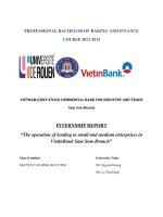
produced from a given amount of inputs. Figure 2-1 and 2-2 illustrate these two approaches. Figure
2-1 demonstrates a firm with two inputs X1 and X2, YY’ is an isoquant which shows every
minimum set of inputs that could be used to produce a given output. If a firm operates on this
isoquant (the frontier), it will be technically efficient in an input-oriented way for the reason that
the inputs amount of this firm is minimized. The iso-cost line CC’ (which can be constructed when
the input-price ratio is known) determines the optimal proportion of inputs in order to archive
lowest cost. Technical efficiency (TE) can be calculated by the percentage rate of OR/OP,
allocative efficiency (AE) equals the percentage rate of OS/OR. The multiplication of AE and TE

Page | 8


expresses the overall efficiency of the firm, called economic efficiency (EE) (i.e.𝐸𝐸 = 𝐴𝐸 × 𝑇𝐸).
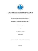
Figure 2-2, illustrate the case where the firm uses one input and produces one output, The f(X)
curve determines the maximum output can be obtained by using each level of input X (the frontier).
The firm will be technical efficient operating on this frontier. In this situation, TE equals BD/DE.

Figure 2 – 1: Input-oriented efficiency

Figure 2 – 2: Output-oriented efficiency

Measurements and analyses of TE were conducted by a huge number of studies with two main
approaches – Data Envelopment Analysis (DEA) and Stochastic Frontier Analysis (SFA). The
next section briefly discusses these two methods.
2. Data Envelopment Analysis (DEA) and Stochastic Frontier Analysis (SFA)
a. Data Envelopment Analysis (DEA)
DEA is a non-parametric method in estimating firm efficiency which was first introduced in
Charnes, Cooper, and Rhodes (1978) with constant return to scale. Later on, it was extended to
allow for decreasing and variable return to scale in Banker, Charnes, and Cooper (1984). Specific
instruction can be found in Banker et al. (1984), Charnes et al. (1978), Fare, Grosskopf, and Lovell
(1994), Färe, Grosskopf, and Lovell (1985) and Ray (2004).
Page | 9


With n firms (called Decision Making Units – DMUs), each firm uses m types of inputs and
produces s types of outputs, the model for DEA following an output-oriented measure is given by:
max ℎ0 =

∑𝑠𝑟=1 𝑢𝑟 𝑦𝑟0

∑𝑚
𝑖=1 𝑣𝑖 𝑥𝑖0

(2.2.1)

Subject to:
∑𝑠𝑟=1 𝑢𝑟 𝑦𝑟𝑗
≤1
∑𝑚
𝑖=1 𝑣𝑖 𝑥𝑖𝑗
𝑢𝑟 , 𝑣𝑖 ≥ 0
With: 𝑗 = 1,2, … , 𝑛; 𝑟 = 1,2, … , 𝑠; 𝑖 = 1,2, … , 𝑚; 𝑥𝑖𝑗 , 𝑦𝑟𝑗 are respectively the ith input and rth
output of jth DMU; 𝑢𝑟 , 𝑣𝑖 are the weights of outputs and inputs which come from the solution of
this maximization problem (Charnes et al., 1978). Using a piece-wise frontier from (Farrell, 1957)
and linear programming algorithm in maximization mathematics, this method constructs a
production frontier. Then, the ratio between outputs and inputs will be brought into account and
compared with the frontier to calculate the efficiency level of each firm.
Only being noticed from 1978, but, for many reasons, DEA has become a popular branch of
efficiency analysis. Wei (2001) described this growing progress by listing five evolvements in
DEA researches. Studies using DEA have been conducted in almost industries, both private and
public sector. Moreover, numerical methods and supporting computer programs have grown in
both number and quality. Over time, new models of DEA have been discussed and established,
such as additive model, log-type DEA model and stochastic DEA model. Besides, the economic
and management background of DEA have been analyzed more carefully and deeply,
strengthening the base for the applications of this model. Mathematical theories related to DEA
have also been promoted by many mathematicians. Those factors gave rise to the progress of both
theoretical improvements and empirical applications of this non-parametric method.
b. Stochastic Frontier Analysis (SFA):
Aigner et al. (1977) and Meeusen and Broeck (1977) suggested the method of production
stochastic frontier to measure firms’ efficiency. The model can be described mathematically as

below:
𝑌𝑖 = 𝑓(𝑋𝑖 , 𝛽)𝑒 𝑣𝑖 −𝑢𝑖

(2.2.2)
Page | 10


with 𝑌𝑖 is output of firm i, 𝑋𝑖 is the vector of inputs, 𝛽 is the vector of parameters, which is to be
estimated. The last two factors: 𝑣𝑖 and 𝑢𝑖 are the two error terms. 𝑣𝑖 is the random statistical noise
and is assumed to have a normal distribution with zero mean. 𝑢𝑖 is a non-negative term indicating
inefficiency, which keeps firm far from producing on its frontier. There are different assumptions
about 𝑢𝑖 ’s distribution such as half normal distribution (Aigner et al., 1977), exponential
distribution (Meeusen & Broeck, 1977), gamma distribution (Greene, 1990) or a non-negative
truncation of 𝑁(𝑚𝑖𝑡, 𝜎 2 ) (Battese & Coelli, 1988, 1992, 1995).
c. Trade-off between DEA and SFA
Being different in approaching method, DEA and SFA have their own advantages and drawbacks.
This implies that when choosing between DEA and SFA, researchers must make some trade-offs.
Being a non-parametric method, DEA is a deterministic approach without the specification of the
production function while SFA is a stochastic technique using econometric (parametric) tools and
requires a model specification (Ray & Mukherjee, 1995). From that key difference, DEA is
considered to be non-statistical, which assumes that the data have no noise. Data noise can come
from measurement errors or random factors which can be controlled by firms. This restrict seems
to be stubborn in realistic situation. SFA is statistical, so it allows and takes into account statistical
noise. In other words, it is more flexible with real world data, in which random factors and error
in collecting is unavoidable. But using SFA requires assumptions about the specification of the
model, functional forms, distribution of parameters and error terms (Wagstaff, 1989). In DEA,
every factor that keeps the firm away from its frontier is regarded inefficiency. While in SFA, the
residual will be decomposed into two components. One part, which is not under the control of the
firm itself, is accounted to be the noise and has the zero mean. The other part, which is known as
the inefficiency, is the weakness of the firm which makes it produce below the frontier. So,

generally, the efficiency measured from SFA will be higher relatively (Ferrier & Lovell, 1990).
DEA has the advantages with the ability to be applied in various complicated condition of
production. Without the requirement of a definite production function, it helps simplifying the
linkage from inputs to outputs of a production process. Without statistical properties, no test can
be used to test DEA’s goodness of fit or specification. In spite of having troubles with model
specification, SFA still has econometric tools to test whether the model is suitable or not. The most
beneficial advantage of SFA is the capability of dealing with statistical noise. Generally, for
industries that the production processes are controlled strictly, DEA seems to be the better choice
Page | 11


of measuring efficiency. This is because the random fluctuation in these industries is minimized
and the production process is very stable (from a given amount of inputs, the number and quality
of outputs is likely to be determined precisely). Meanwhile, SFA tends to be suitable for industries
in which noise is inevitable. Firms in those industries have to bear the impacts from random
fluctuations. In the case of this thesis, firms in metal manufacturing industries are influenced by
from the markets of both inputs and outputs, both domestic and abroad and changes in policies.
For those natures of the industries the thesis analyzed, SFA is the better model to be applied. The
next part discusses in detail SFA method, both cross-sectional and panel data models.
3. The cross-sectional Stochastic Frontier Model:
The cross-sectional stochastic frontier model in Aigner et al. (1977) can be describe as:
𝑦𝑖 = 𝑓(𝑥𝑖 , 𝛽) + 𝑣𝑖 − 𝑢𝑖

(2.3.1)

with 𝑣𝑖 is the random noise and 𝑢𝑖 is technical inefficiency (𝑢𝑖 ≥ 0). To distinguish these two
components of residual, some assumptions are necessary. The first assumption is about the
distribution of 𝑢𝑖 while 𝑣𝑖 follows a symmetric normal distribution. For the reason that 𝑢𝑖
represents the distance from the frontier which keeps firms below the frontier, its value is nonnegative. As mentioned above, the distribution that is suggested includes half normal distribution
(Aigner et al., 1977), exponential distribution (Meeusen & Broeck, 1977), gamma distribution

(Greene, 1990) or a non-negative truncation of 𝑁(𝑚𝑖𝑡, 𝜎 2 ) (Battese & Coelli, 1988, 1992, 1995).
Both two main estimation methods of econometric can be used to deal with technical inefficiency
calculation – Ordinary Least Squares (OLS) and Maximum Likelihood (ML). But for the fact that
the error term 𝜀 includes two components, that is: 𝑢 with an asymmetric distribution and 𝑣 with a
symmetric distribution, so 𝜀 will not have normal distribution. Since 𝜀 = 𝑣 − 𝑢 then 𝜇𝜀 = −𝜇𝑢 .
This makes the intercept in OLS bias downward. To clarify, we consider a regression with just the
intercept 𝛼: 𝑦 = 𝛼 + 𝜀, then the estimator for 𝜀 will be 𝑦̅. From the equation above, 𝑝𝑙𝑖𝑚(𝑦̅) =
𝛼 + 𝜀, which does not equal to 𝛼. Winsten (1957) suggested an method called Corrected Ordinary
Least Squares (COLS), Afriat (1972) and Richmond (1974) offered the method of Modified
Ordinary Least Squares (MOLS) to solve this bias problem. Those two methods correct or modify
the intercept upward by add up the maximum or average value of OLS residuals. COLS and MOLS
have some problems, such as non-statistical meaning estimates (Mastromarco, 2007). ML,
however, has some asymptotic properties and is able to deal with asymmetrically distributed
residual, is used frequently than OLS.
Page | 12


With technical inefficiency (𝑢) following a half-normal distribution i.e. 𝑢~𝑁 + (0, 𝜎𝑢2 ) (Aigner et
al., 1977) the log-likelihood function is:
𝐼

𝐿𝑛 𝐿(𝑌|𝛽, 𝜎, 𝜆) = − 2 ln (

𝜋𝜎2
2

) + ∑𝐼𝑖=1 𝑙𝑛Φ (−

𝜀𝑖 𝜆
𝜎

1

) − 2𝜎2 ∑𝐼𝑖=1 𝜀𝑖2

(2.3.2)

with 𝜎 2 = 𝜎𝑣2 + 𝜎𝑢2 and 𝜆 = 𝜎𝑢2 ⁄𝜎𝑣2 . If 𝜆 = 0, the firm is fully efficient. If 𝜆 = 1, it is totally
inefficient. In the equation above, 𝑦 is a vector of logarithm of outputs; 𝜀𝑖 = 𝑣𝑖 − 𝑢𝑖 = ln 𝑞𝑖 − 𝑥𝑖′ 𝛽
and Φ(𝑥) is the cumulative distribution function (cdf) of a random variable which follows N(0,1)
distribution at x (Coelli et al., 2005). This function can be solved using an iterative optimization
procedure in Judge, Hill, Griffiths, Lutkepohl, and Lee (1982) as cited in Coelli et al. (2005).
Log-likelihood function with exponential distribution can be described as:
𝜎2

−𝜀

𝜀

𝑗
𝑗
𝑁
−1
ln 𝐿(𝑌|𝛼, 𝛽, 𝜆, 𝜎 2 ) = −𝑁 (𝑙𝑛 𝜎𝑢 + 2𝜎𝑣2 ) + ∑𝑁
𝑗=1 𝑙𝑛 Φ ( 𝜎 − 𝜆 ) + ∑𝑗=1 𝜎
𝑢

𝑣

𝑢

(2.3.3)

with 𝑢~𝐸𝑥(𝜃); 𝜃 = 𝜎𝑢−1 .
The case of truncated normal distribution i.e. 𝑢~𝑁 + (𝜇𝑢, 𝜎𝑢2 ) has the log-likelihood function:
𝑁

ln 𝐿(𝑌|𝛼, 𝛽, 𝜆, 𝜎

2)

−𝜇𝜆−1 − 𝜀𝑗 𝜆
−𝑁
𝜋
−𝜇
=
ln ( ) − 𝑁𝑙𝑛(𝜎) − 𝑁Φ ( ) + ∑ ln Φ (
)
2
2
𝜆𝜎
𝜎
𝑗=1

1

2
− 2𝜎2 ∑𝑁
𝑗=1 𝜀𝑗

(2.3.3)

Log likelihood function for Stochastic Frontier Model with gamma distribution of u can be found
in Greene (1990):
ln 𝐿 = ∑𝑖(𝑃𝑙𝑛Θ − 𝑙𝑛Γ(𝑃) +

Θ2 𝜎 2
2

+ Θ𝜀𝑖 + 𝑙𝑛𝑃𝑟𝑜𝑏[𝑄 > 0|𝜀𝑖 ] + ln ℎ[𝑃 − 1, 𝜀𝑖 ])

(2.3.4)

with Θ and P are two parameters of a gamma distribution.

Page | 13


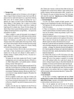
Figure 2 – 3: Distribution of technical inefficiency

Figure (2 - 3) illustrates the probability density function of four types of distribution of 𝑢 visually.
Obviously, there are restrictions with gamma, exponential and half-normal distribution. With these
distributions, because most observations locate in the area has low value of u (technical
inefficiency), one can conclude that the level of efficiency of firms is rather high (the inefficiency
level is low). Put differently, most firms are highly efficient. This can be untrue with many
industries, in which high efficiency is not realistic. Truncated normal distribution is more flexible
when it allows the allocation of inefficiency to almost positive point. Therefore it can be used to
describe 𝑢 better.
Consider a Cobb-Douglas production function as:
ln 𝑌𝑖 = 𝛽 ln 𝑋𝑖 + 𝑣𝑖 − 𝑢𝑖

(2.3.5)

The technical inefficiency level of a firm can be calculated as the ratio of observed output (𝑌𝑖 ) to
maximum feasible output 𝑌 ∗ which is the output when the firm is fully efficient or the value of 𝑢𝑖
is zero.
𝑌

𝑇𝐸𝑖 = 𝑌 ∗𝑖 =

𝑒 (𝛽 ln 𝑋𝑖 +𝑣𝑖 −𝑢𝑖 )
𝑒 (𝛽 ln 𝑋𝑖 +𝑣𝑖 )

= 𝑒 (−𝑢𝑖 )

(2.3.6)

With 𝑢𝑖 follows the 𝑁(𝑚𝑖, 𝜎 2 ) distribution in Battese and Coelli (1995), the parameter for
inefficiency (or, in other words, also efficiency) can be analyzed with some determinants with the
regression equation follow:
Page | 14


𝑚𝑖 = 𝛿0 + 𝑍𝑖 𝛿 + 𝜔𝑖

(2.3.7)

With 𝑍𝑖 is the vector of determinants of 𝑚𝑖 and 𝛿 is the vector of parameters that need to be
estimated. The distribution of 𝜔𝑖 is the truncation of the normal distribution 𝑁(0, 𝜎 2 ) (Battese &
Coelli, 1995). This is called Technical Inefficiency Model and can be estimated simultaneously

with the Stochastic Frontier.
4. Stochastic frontier model with panel data
There are three problems arising while we use stochastic frontier model with cross sectional data
(Schmidt & Sickles, 1984). The first is the inconsistency in estimating technical inefficiency. Most
studies in this field uses the method in Jondrow, Lovell, Materov, and Schmidt (1982) to predict
the technical inefficiency level for each firm in the sample. The formula is:
𝐸(𝑢|𝜀) = 𝜇∗ + 𝜎∗

𝜇
𝑓(− ∗ )
𝜎∗

𝜇
1−𝐹(− ∗ )

(2.4.1)

𝜎∗

where 𝑓 and 𝐹 are the standard normal density and cumulative density function respectively, 𝜇∗ =
−𝜎𝑢2 𝜀 ⁄𝜎 2 , 𝜎∗2 = 𝜎𝑢2 𝜎𝑣2 ⁄𝜎 2 and 𝜎 2 = 𝜎𝑢2 + 𝜎𝑣2 . For the reason that 𝜇∗ and 𝜎∗ are unknown so their
estimator 𝜇̂ ∗ and 𝜎̂∗ are used instead which leads to some sampling bias. In principle, one must
take into account this bias but it is very complicated to do. This kind of bias disappears
asymptotically and can be ignored with large sample. However, essentially, technical inefficiency
is independent of sample size. So the level of technical inefficiency level will be estimated
inconsistently (Schmidt and Sickles, 1984). The second is the ambiguity in the distribution of 𝑢,
which is necessary to guarantee an independence between technical inefficiency (𝑢) and statistical
noise (𝑣). Without a stubborn distribution assumption, it is impossible to decompose the overall
error term (𝜀) into inefficiency (𝑢) and statistical noise (𝑣). However, with cross-sectional data,
the robustness of the assumption is hard to test. The third problem is the assumption of the

uncorrelatedness of u with other regressors in the model. This problem of endogeneity causes
biases in the model. Schmidt and Sickles (1984) suggests that the endogeneity is unavoidable
because in the long-run the firm realizes its inefficiency level and adjusts the use of inputs to be
more efficient.
Panel data models (with data from N firms in T periods) can help avoid these three weaknesses
(Greene, 2008). Firstly, more observation overtime (the ideal case is when we have long enough
Page | 15


time series data T→∞) helps estimate the technical inefficiency more consistently. Secondly, by
isolation and treating technical inefficiency as fixed effect, the model using panel data is
distribution free (the distribution assumption is now optional) (Greene, 2008). Finally, the
assumption of uncorrelatedness is also relaxed because some panel models can take into account
the effects of this correlation. The next section describes in detail those panel data stochastic
frontier models which have been developed over a long period since its first appearance.
4.1 Time-invariant models
a. Within estimation with fixed effects and GLS estimation with random effects from
Schmidt and Sickles (1984)
From those discussion above, Schmidt and Sickles (1984) suggests the use of panel data to estimate
technical inefficiency (time invariant) both with fixed and random effects. The model is described
as:
ln 𝑦𝑖𝑡 = 𝛼 + 𝑋𝑖𝑡′ 𝛽 + 𝑣𝑖𝑡 − 𝑢𝑖

(2.4.2)

*Note: Schmidt and Sickles (1984) use a log-linear function.

with 𝑣𝑖𝑡 is uncorrelated with 𝑋𝑖𝑡′ 𝛽 and 𝑢𝑖 . The within estimator uses dummy variables to estimate
separate intercepts for each firm which stand for its own technical inefficiency. This method has
advantages because it need neither an assumption about the uncorrelatedness between 𝑢 and other

variables nor an assumption about 𝑢’s distribution. After calculating, each firm’s effect is
compared with the highest in the sample and inefficiency is estimated as 𝑢̂𝑖 = max(𝛼̂𝑖 ) − 𝛼̂𝑖 . The
authors suggests a large number of firms to have exact estimate of the most efficient firm in the
sample (the ideal case is with an extensive number of firms over a considerable number of time
periods). For the fact that this method is simply a fixed effects estimation using panel data, it
includes in technical inefficiency the effects of time-invariant but firm-varying effects (as Schmidt
and Sickles (1984) mentioned, it can be capital stock for example – if the value of capital stock
stays unchanged overtime, fixed effects model will include it in the value of firm’s specific
intercept) which cannot be considered as inefficiency.
From the weaknesses of the within estimator mentioned above, the authors suggests assumptions
about the uncorrelatedness of 𝑢 and 𝑋𝑖𝑡′ 𝛽, based on which we can conduct GLS estimation to
estimate 𝑢 better. The better point from this method comes from the ability to separate the timeinvariant regressor which within estimator cannot. However, the stubborn assumption needs to be
Page | 16


tested. Given the matter of uncorrelatedness and distribution assumptions, the authors suggests
other two methods. The first is the estimation of Hausman and Taylor (1981) which relaxes the
uncorrelatedness assumption and the second is the maximum likelihood estimation which are more
advanced given a specific distribution of 𝑢.
The two model considered above is two of some simplest approaches to the concept of technical
efficiency. With their criticism about the inconsistency in estimating technical inefficiency level,
they suggest the use of fixed and random effects model which give more consistent estimate of
technical inefficiency in case T is large with a given N. However, the lack of a distribution makes
it hard to estimate the true inefficiency apart from other firm-specific factors. Back in time in Pitt
and Lee (1981), a half normal distribution with maximum likelihood estimation is described in the
next section.
b. The model with time-invariant efficiency in Pitt and Lee (1981)
In this paper, the panel data from the Indonesian weaving industry was used to estimate technical
inefficiency level and its sources. The hypothesis of whether technical inefficiency is timeinvariant or time-varying was tested using three different models. Three cases were suggested by
the authors. The first case is when 𝑢 is fixed through time and only varies among individuals,

which means it is indexed by 𝑖 only (𝑢𝑖 ) as described below:
𝑦𝑖𝑡 = 𝑥𝑖𝑡 𝛽 + 𝑣𝑖𝑡 − 𝑢𝑖

(2.4.3)

*Note: Pitt and Lee (1981) use a linear function.

In the second case, technical inefficiency is independent of time and among individuals, which
leads back to the cross-sectional model as in Aigner et al. (1977). That is:
𝑦𝑖𝑡 = 𝑥𝑖𝑡 𝛽 + 𝑣𝑖𝑡 − 𝑢𝑖𝑡

(2.4.4)

With 𝐸(𝑢𝑖𝑡 𝑢𝑖𝑡 ′ ) = 0 and 𝐸(𝑢𝑖𝑡 𝑢𝑗𝑡 ′ ) = 0 for all 𝑖 ≠ 𝑗 and 𝑡 ≠ 𝑡′.
The final case is the intermediate of these two when the technical inefficiency is assumed to be
correlated with time. That is:
𝑦𝑖𝑡 = 𝑥𝑖𝑡 𝛽 + 𝑣𝑖𝑡 − 𝑢𝑖𝑡

(2.4.5)

With 𝐸(𝑢𝑖𝑡 𝑢𝑖𝑡 ′ ) ≠ 0 and 𝐸(𝑢𝑖𝑡 𝑢𝑗𝑡 ′ ) = 0 for all 𝑖 ≠ 𝑗 and 𝑡 ≠ 𝑡′.
Page | 17


The first and second models are estimated using maximum likelihood method while the
intermediate model is estimated with generalized least squares (for the reason that the maximum
likelihood procedure for the last case is intractable). Comparing between two first models and
model three is conducted by a 𝜒 2 test which can be found in Jöreskog and Goldberger (1972). The
test suggests that the last model is appropriate (which implies technical inefficiency is time
varying). The measure of technical inefficiency for each firm is not mention in the paper, however,

can be done by the method of Jondrow et al. (1982) which infers the value of each 𝑢𝑖 from the
value of each 𝜀𝑖 .
Although the last model is shown to be more precise, it does not take into account the distribution
of technical inefficiency. Moreover, it supplies no measure of inefficiency. Thus, generally, the
idea proposed by Pitt and Lee (1981) hinges around a model with time-invariant inefficiency
following half normal distribution and suggests further research into time varying inefficiency.
However, as mentioned above, a half normal distribution is sometimes unreasonable. Battese and
Coelli (1988) suggests a more general distribution of 𝑢 – the truncated normal distribution. The
model is discussed in detail in the next section.
c. The model with truncated normal distribution in Battese and Coelli (1988)
Battese and Coelli (1988) proposes a model in that technical inefficiency follows a truncated
normal distribution which is developed in Stevenson (1980) for the estimation of stochastic
production frontier. For the availability of data (3 years), the authors make the assumption of timeinvariant inefficiency. The new distribution is 𝑁 + (𝜇, 𝜎𝑢2 ). It is more general than the old ones (half
normal, which is introduced in Pitt and Lee (1981) and Schmidt and Sickles (1984)) because when
𝜇 = 0, the distribution becomes half normal. With development in calculating the likelihood
function from Stevenson (1980), the model is estimated with maximum likelihood method. The
model can be described as:
ln 𝑦𝑖𝑡 = 𝛼 + 𝛽𝑙𝑛𝑥𝑖𝑡 + 𝑣𝑖𝑡 − 𝑢𝑖

(2.4.6)

*Note: Battese and Coelli (1988) use a Cobb-Douglas function

An extensive contribution of this paper to the field of stochastic frontier is its approach in
estimating technical efficiency both in the industry level and firm level for the logarithmic case
(the Cobb-Douglas functional form in the study). Instead of using the mean of technical
inefficiency - 𝐸(𝑢) and calculating the efficiency level as 1 − 𝐸(𝑢) in Jondrow et al. (1982), the
Page | 18

authors suggests that technical efficiency level should be attained in form of exp(−𝑢) in the
logarithmic case. The formula of technical efficiency level is then clarified with the properties of
truncated distribution of 𝑢.
A common suggestion from the studies mentioned above is the research direction into time varying
characteristics of 𝑢. Pitt and Lee (1981) base on their empirical evidences to suggest further
research about time varying technical inefficiency. Schmidt and Sickles (1984) also state that firms
will recognize their inefficiency level in the long-run and change themselves to be more efficient.
The lack of a long-period data makes Battese and Coelli (1988) assume 𝑢 to be fixed through time,
however in their hint for future research, they also suggest other models that allow inefficiency to
vary overtime. To relax the inflexible assumption of time-invariant inefficiency, models with time
varying inefficiency arise. The next section considers those models.
4.2 The time varying models
a. The model of Cornwell et al. (1990)
As mentioned above, the problems of technical inefficiency’s distribution and that whether it is
uncorrelated with inputs are treated differently among researches. Once those assumptions about
uncorrelatedness and distribution are made, they easily look too stubborn and become a weakness
of the study. Panel data can help relax those assumption but in the cost of treating technical
inefficiency as fixed through time. Once again, the assumption of a time-invariant efficiency is too
strong (Cornwell et al., 1990). By regarding firm effect as a function of time with parameters alter
across firms, Cornwell et al. (1990) create a model that changes the fixed firm-effect into flexible
firm effect which can be varied overtime. The model can be described as:
ln 𝑦𝑖𝑡 = 𝛼𝑖𝑡 + 𝛽 ln 𝑋𝑖𝑡 + 𝑣𝑖𝑡

(2.4.7)

*Note: Cornwell et al. (1990) use a Cobb-Douglas function.

with 𝛼𝑖𝑡 is time varying firm effects which follows a function of time. The authors mentions a
quadratic function of time with parameters vary across firms described as
𝛼𝑖𝑡 = 𝜃𝑖1 + 𝜃𝑖2 𝑡 + 𝜃𝑖3 𝑡 2

(2.4.8)

which allows firm effects change across firms and overtime. The model can be estimated by within
estimator, GLS or efficient instrumental estimator. The residuals after being estimated, are
regressed on a quadratic function of time. Firm specific temporal effect 𝛼𝑖𝑡 then is estimated using
Page | 19


the coefficients of the latter estimation. Using the method similar to the one in Schmidt and Sickles
(1984), the authors calculated firm specific temporal inefficiency level:
𝑢𝑖𝑡 = 𝛼̂𝑡 − 𝛼̂𝑖𝑡

(2.4.9)

with 𝛼̂𝑡 = 𝑚𝑎𝑥𝑗 (𝛼̂𝑗𝑡 ) which is a comparing the specific effect of each firm to the most efficient
firm (in that year).
This model well adapts to time varying technical inefficiency. However, by using parameters that
vary across firms (𝑁 × 3 parameters), its degree of freedom is heavily affected in small sample
(especially sample with small T). The model of Kumbhakar (1990), Battese and Coelli (1992) and
Lee and Schmidt (1993) which include less parameters and uses a specific distribution of 𝑢 to
capture the time varying inefficiency of firms will be discussed in the following section.
b. The model of Kumbhakar (1990), Battese and Coelli (1992) and Lee and Schmidt (1993)
Kumbhakar (1990) considers the time varying inefficiency as a function of time and time invariant
inefficiency. The model can be described as:
ln 𝑦𝑖𝑡 = 𝛼 + 𝛽 ln 𝑋𝑖𝑡 + 𝑣𝑖𝑡 − 𝑢𝑖𝑡

(2.4.10)

*Note: Kumbhakar (1990) use a Cobb-Douglas function.

with 𝑢𝑖𝑡 = 𝛾(𝑡)𝑢𝑖 where 𝑢𝑖 is fixed through time but varied across firms and 𝑢𝑖 follows a half
normal distribution. The suggested time function is:
𝛾(𝑡) = (1 + exp(𝑏𝑡 + 𝑐𝑡 2 ))−1

(2.4.11)

The fact that 𝛾(𝑡) ≥ 0 makes 𝑢𝑖𝑡 always positive in the production.
The values of 𝑏 and 𝑐 decide 𝛾(𝑡) to be monotonically increasing or decreasing and to be concave
or convex. Thus, the data which is used to estimate the model can determine the time-behavior of
𝛾(𝑡) and also 𝑢𝑖𝑡 . Then we can easily test the functional form of 𝛾(𝑡) by a LR test with the null
hypothesis 𝑏 = 0, 𝑐 = 0 or 𝑏 = 𝑐 = 0. The model then is estimated by ML method with the
likelihood function as given in the paper. After estimating 𝛾̂(𝑡) and 𝑢̂𝑖 , temporal technical
inefficiency for each firm is calculated as 𝑢̂𝑖𝑡 = 𝛾̂(𝑡) × 𝑢̂𝑖 .
Having the same thought as in Kumbhakar (1990), the model in Battese and Coelli (1992) also
considers the form of technical inefficiency as 𝑢𝑖𝑡 = 𝛾(𝑡)𝑢𝑖 with the form of 𝛾(𝑡) =
exp[−𝜂(𝑡 − 𝑇)] and 𝑢𝑖 𝑖𝑖𝑑 |𝑁(𝜇, 𝜎𝑢2 )| (truncated normal distribution at zero). The value of 𝜂
Page | 20


determine the time behavior of technical inefficiency. When 𝑡 increases, 𝑢𝑖𝑡 will increase, remain
constant or decrease if 𝜂 < 0, 𝜂 = 0 or 𝜂 > 0 repectively. Thus the functional form of technical
inefficiency can be decided by the data. This approach, however is simpler and uses less
parameters than the one in Kumbhakar (1990).
The model in Lee and Schmidt (1993) replace the time function in those two previous studies by
a set of dummy variables 𝜃𝑡 . The model can be described as:
𝑦𝑖𝑡 = 𝑋𝑖𝑡 𝛽 + 𝜃𝑡 𝑢𝑖 + 𝑣𝑖𝑡

(2.4.12)

*Note: Lee and Schmidt (1993) use a linear function.

with 𝑢𝑖 is firm’s time invariant technical inefficiency. The authors suggest that by doing this, the
time pattern is not restricted to a specific functional form of time. However the number of
parameters can be large (even though smaller than the one in Cornwell et al. (1990)) in the case T
is large, thus the authors recommend this method in the case the time-series is not too long. Since
it does not use any distribution of technical inefficiency, the method of within estimator and GLS
is applied to estimate the model.
Generally, the three models mentioned above adapts well in dealing with time varying technical
inefficiency and relax the strong time-invariance assumption. However, they do not consider the
matter of determinants of technical inefficiency. This matter is first regarded in the study of Pitt
and Lee (1981) with the purpose of finding the source of technical inefficiency. This kind of model
which is called as technical inefficiency effects model (TIEM) has been developed through the
researches of Kumbhakar, Ghosh, and McGuckin (1991), Reifschneider and Stevenson (1991) and
Huang and Liu (1994). The next section will describe the model of Battese and Coelli (1995), a
popular model which includes both stochastic frontier model and technical inefficiency effects
model.
c. The model of Battese and Coelli (1995) with technical inefficiency effects model
The model suggested in this paper includes a stochastic frontier model and a technical inefficiency
effects model. Theoretically, the stochastic frontier model estimates technical inefficiency of firms
from the data of outputs and inputs and then the technical inefficiency effects model regresses 𝑢
on other variables which can be considered as explanatory factors associated with 𝑢. The formula
of stochastic frontier model for panel data can be described as:

Page | 21


𝑌𝑖𝑡 = exp(𝑥𝑖𝑡 𝛽 + 𝑉𝑖𝑡 − 𝑈𝑖𝑡 )

(2.4.13)

*Note: Battese and Coelli (1995) use a Cobb-Douglas function.

with 𝑥𝑖𝑡 is a vector of value of a specific functional form, 𝑉𝑖𝑡 is symmetric normal distributed
statistical noise. 𝑈𝑖𝑡 follows a truncated normal distribution with mean 𝑧𝑖𝑡 𝛿 and variance 𝜎 2 with
𝑧𝑖𝑡 is a vector of explanatory variables which can be considered as sources of technical
inefficiency.
The two models are estimated simultaneously using maximum likelihood method given the
truncated normal distribution of 𝑢. In this paper, Battese and Coelli use micro panel data of India
villages to apply the model. A time variable is included in the stochastic frontier model to take into
account the technical progress (Hicksian neutral technological change) while a time variable is
used in the technical inefficiency model to imply the time varying characteristic of 𝑢 (here is a
linear correlation). With similar procedure in their papers in 1988, 1992 and 1993, the authors use
a log likelihood test to examine the existence of technical inefficiency, functional form of
stochastic frontier model and technical inefficiency effects model.
Having the ability to take into account the impacts of explanatory factors on technical inefficiency,
the (Battese & Coelli, 1995)’s model is applied widely to analyze technical efficiency and its
determinants. This application is useful in the case of discovering factors that benefit firms in
gaining efficiency. Thus, become a powerful tool in policy recommendation. However, the fact
that technical inefficiency can be explained by other factors raises the problem of biases in
estimating the whole model. Greene (2005) seriously criticizes this matter and proposes a new
approach which called “true” fixed effects model and “true” random effects model. Those models
are described in detail below.
d. “True” fixed effects model and “true” random effects model (Greene, 2005)
Greene (2005) mentions two shortcomings of those fixed effects and random effects approaches
mentioned above. The first is the strong assumption about the time pattern of technical
inefficiency. The model of Pitt and Lee (1981), Schmidt and Sickles (1984) and Battese and Coelli
(1988) both assume a time invariant technical inefficiency. This assumption becomes too strong,
especially in the case of using panel data with large number of time periods. Cornwell et al. (1990)
proposes a model to deal with this problem by using a time function with parameters change across

firms. By this way, the number of parameters is large and this makes the model inefficient. Later
Page | 22


papers such as Battese and Coelli (1992), Lee and Schmidt (1993) and Kumbhakar (1990) solve
the problem by adding a time behavior function 𝑔(𝑡) so 𝑢𝑖𝑡 = 𝑔(𝑡)𝑢𝑖 . Despite the various
functional forms of 𝑔(𝑡), the assumption that technical inefficiency follows a specific pattern of
time, again, seems to be strong either (Greene, 2005).
The second matter is the assumption that 𝑢𝑖𝑡 is uncorrelated with other variables in the model. The
previous fixed effects model does not need this assumption. By imposing a separate intercept for
each firm, the “firm effect” now is not correlated with other variables. However, Greene criticizes
that by doing this, one can only compute technical inefficiency by comparing with the “best” firm
in the sample. Besides, he also states that “firm effect” from this method includes heterogeneity
that is not related to inefficiency. In his view, technical inefficiency needs not contain time
invariant effects and should vary freely through time (Greene, 2008). This kind of heterogeneity
is also considered in the study of Farsi, Filippini, and Kuenzle (2003) as factors beyond the control
of firms. The authors give the examples of factors that belongs to business environment (for
example: network effects in network industries) or relates to output characteristics such as the
severity of illness in healthcare industry or the demand fluctuations in electricity utilities. In
healthcare industry, different hospitals must treat different kinds of disease with different severity
level. If we take number of lives saved by a hospital as the representative of output, then this
number will be low in the hospitals which mainly treat minor diseases and vice versa. Thus, those
hospitals will be closer to the frontier than others with major diseases. One can conclude that the
hospitals treating minor diseases are more efficient than the hospitals treating major diseases. If
we let them cure the same amount of patients that have the same level of severity, we cannot assure
which group will save more. Therefore, taking those effects into technical efficiency level is not
reasonable. From those ideas, Greene (2005) suggests “true” fixed and random effects model
which separate that latent heterogeneity from inefficiency.
“True” fixed model is described as:
𝑦𝑖𝑡 = 𝛼𝑖 + 𝛽 ′ 𝑥𝑖𝑡 + 𝑣𝑖𝑡 − 𝑢𝑖𝑡

(2.4.14)

with 𝛼𝑖 is the firm specific constant. Greene also introduces a maximization method that can help
estimating simultaneously all coefficients by maximum likelihood which uses a specific
distribution of 𝑢. Meanwhile the “true” random effects model can be written as:
𝑦𝑖𝑡 = (𝛼 + 𝑤𝑖 ) + 𝛽 ′ 𝑥𝑖𝑡 + 𝑣𝑖𝑡 − 𝑢𝑖𝑡

(2.4.15)
Page | 23


*Note: the functional form of production function in equation (2.4.14) and (2.4.15) are the ones that were used in
Greene (2005) to introduce their model. In their examples, they use the Cobb-Douglas form.

with 𝑤𝑖 is a random constant term that varies across firms.
As we can see, those panel data models mentioned above can be divided into two groups by types
of approach. Those with fixed effects approach as the fixed effects model in Schmidt and Sickles
(1984), Cornwell et al. (1990), Lee and Schmidt (1993) and Greene (2005) do not require
assumptions on the uncorrelatedness between technical inefficiency and other parts of the model.
Those with random effects approach such as the models in Schmidt and Sickles (1984) (random
effects model), Pitt and Lee (1981), Battese and Coelli (1988, 1992, 1995), Kumbhakar (1990) and
“true” random effects model in Greene (2005) require technical inefficiency to be uncorrelated
with the rest of the model. People can also divide them into time invariant models and time varying
models as mentioned above. Coming from different points of view, they have their own strengths
and weaknesses that make them suitable to different situations.
The literature on cross-sectional data stochastic frontier model is quite consistent. Its simplicity
and weaknesses attract less attention. When the need of a more careful analysis into the nature of
firm’s efficiency arises and the data in panel form are now attainable widely, researchers tend to
rely on panel data models despite their complicatedness. Like what I mentioned about my intention

for this thesis, I will only apply those models with panel data in my empirical process. The purpose
is to compare them relatively to each other, to find out differences that make them more or less
suitable in specific circumstances. The methodology will be described particularly in the section
below.

Page | 24


CHAPTER III: METHODOLOGY
1. Overview of Vietnamese metal manufacturing industry
Firms in the sample used in this study are divided into two categories: basic metal manufacturing
firms and fabricated metal manufacturing (except machinery and equipment) firms according to
their main products. Details for this classification can be found in International Standard Industrial
Classification of All Economic Activities (ISIC), Revision 4. Firms in the first group are involved
in the activities of smelting and refining ferrous and non-ferrous metals. Those firms use
metallurgic techniques with the materials from mining industry such as metal ore, pig or scrap.
Taking part in this industry need large investments in physical assets. Thus, in this sample of small
and medium enterprises, this group takes only 9% of the numbers of firms. The second group
manufactures structural metal products, metal container-typed objects and steam generators.
Producing more popular products, this group takes about 91% of the number of firms.
The metal manufacturing industry in Viet Nam has many potentials due to the high demand of
metal products for daily using, production and construction. In Vietnamese young developing
economy, metal manufacturing industry is still immature and most products are used for
construction. According to World Steel Association, about 80% of iron and steel materials are used
for construction. Besides, the domestic rising demand of metal materials of machinery, motor and
automobile and other consumer goods manufacturing can also be considered as important
condition of development of metal manufacturing industry. However, along with the depressed
situation of Vietnamese economy in the recent year, metal manufacturing industry also has many
difficulties. The investment cut in public construction due to government budget deficit strongly
decreases the demand of metal materials for construction. According to Vietnamese Steel

Association, steel consumption fell about nine percent in 2012. The rising price of inputs such as
electricity, water and labor cost also imposes many hardships on this industry.
Due to the importance of metal manufacturing industry, this study is conducted with the objective
of analyzing technical efficiency level of firms in this sector. However, most observations in this
sample are micro and household firms (74.5%) and the number of medium sized firms take only
four percent. Moreover, due to the availability of data, the dataset used here is in the period of
2005 to 2009, during which economic conditions may be different from the current situation.
Because of those reasons, there should be high probability of sample bias if this study gives
Page | 25