The relationship between financial development and household welfare case study in five asian countries
Bạn đang xem bản rút gọn của tài liệu. Xem và tải ngay bản đầy đủ của tài liệu tại đây (1.65 MB, 66 trang )
UNIVERSITY OF ECONOMICS
INSTITUTE OF SOCIAL STUDIES
HO CHI MINH CITY
THE HAGUE
VIETNAM
THE NETHERLANDS
VIETNAM-NETHERLANDS PROGRAMME FOR MASTER IN
DEVELOPMENT ECONOMICS
THE RELATIONSHIP BETWEEN
FINANCIAL DEVELOPMENT AND
HOUSEHOLD WELFARE:
CASE STUDY IN FIVE ASIAN COUNTRIES
By
PHAN THI KHANH VAN
This paper was submitted in partial fulfillment of the requirements for
Master’s degree in Development Economics
Ho Chi Minh City, July 2013
UNIVERSITY OF ECONOMICS
INSTITUTE OF SOCIAL STUDIES
HO CHI MINH CITY
THE HAGUE
VIETNAM
THE NETHERLANDS
VIETNAM-NETHERLANDS PROGRAMME FOR MASTER IN
DEVELOPMENT ECONOMICS
THE RELATIONSHIP BETWEEN
FINANCIAL DEVELOPMENT AND
HOUSEHOLD WELFARE:
CASE STUDY IN FIVE ASIAN COUNTRIES
By
PHAN THI KHANH VAN
Academic supervisor
Dr. DUONG NHU HUNG
Thispaper was submitted in partial fulfillment of the requirements for
Master’s degree in Development Economics
Ho Chi Minh City, July 2013
CONTENTS
ACKNOWLEDGEMENT ..................................................................................................... iii
ABSTRACT ............................................................................................................................ iv
ABBREVIATION .................................................................................................................... v
LIST OF FIGURES ................................................................................................................ vi
LIST OF TABLES .................................................................................................................. vi
CHAPTER I: INTRODUCTION ........................................................................................... 1
1. Problem statement ............................................................................................................... 1
2. Research objectives ............................................................................................................. 3
3. Research questions .............................................................................................................. 4
4. Justification of the study ..................................................................................................... 4
5. Scope of the study ............................................................................................................... 4
6. Structure of the study .......................................................................................................... 4
CHAPTER II: LITERATURE REVIEW ............................................................................. 5
1. Definitions of key concepts ................................................................................................ 5
1.1. Financial development ................................................................................................. 5
1.2. Household welfare and Poverty ................................................................................... 5
2. Theoretical literature ........................................................................................................... 6
2.1. Direct relationship ........................................................................................................ 7
2.2. Indirect relationship ..................................................................................................... 8
3. Empirical studies ................................................................................................................. 9
CHAPTER III: ECONOMETRICS REVIEW................................................................... 12
1. Stochastic Process, Stationarity and Random Walks ........................................................ 12
2. Unit Root Test ................................................................................................................... 13
3. Cointegration..................................................................................................................... 13
4. Granger Causality Test ..................................................................................................... 14
5. Panel Unit Root Test ......................................................................................................... 15
6. Panel Cointegration ........................................................................................................... 16
[i]
7. Instrumental Variables Regression (IV) ........................................................................... 18
8. Generalized method of moments (GMM)......................................................................... 19
CHAPTER IV: DATA AND RESEARCH METHODOLOGY ....................................... 22
1. Data ................................................................................................................................... 22
2. Research methodology ...................................................................................................... 23
CHAPTER V: ANALYSIS RESULTS ................................................................................ 26
1. Data descriptions ............................................................................................................... 26
2. Empirical results ............................................................................................................... 31
CHAPTER VI: CONCLUSIONS AND POLICY IMPLICATIONS ............................... 36
1. Conclusions ....................................................................................................................... 36
2. Policy implications............................................................................................................ 37
3. Limitations and directions for further studies ................................................................... 38
3.1. Limitations ................................................................................................................. 38
3.2. Directions for further studies ..................................................................................... 39
REFERENCES ...................................................................................................................... 40
APPENDICES.......................................................................................................................... a
Appendix 1: Description of FD and PR variables (1998-2011) ............................................. a
Appendix 2: Panel Unit Root Test of variables ...................................................................... b
Appendix 3: Pedroni Cointegration Test ................................................................................. j
Appendix 4: GMM................................................................................................................. m
[ii]
ACKNOWLEDGEMENT
The study would be done successfully thank to the beautiful assistance and guidance of
everybody who are always with me during the research period.
First, I would like to express my deepest appreciation to The Board of Management and
Theoretical Supervision of this program. In fact, I would like to send sincere thanks to Dr.
Nguyen Trong Hoai, Dr. Pham Khanh Nam who give me a very first step guidance doing this
study (theoretical review and techniques understanding) and give me a piece of advice when I
got in stuck with my study. Besides that, I also thank to Dr. Duong Dang Thuy, who has given
me theoretical advice and introduced me to Dr. Le Van Chon for intensive support.
Moreover, I would like to express my gratitude to Dr. Le Van Chon and Dr. Phung
Thanh Binh who supported my study and my mind when I lost inspiration during research
period. Not only the teaching staff but also the class MDE 17 classmates are those I really
appreciate. Thanks to their care, their understanding and their sharing, I know exactly what I
should do.
The more importantly, I would like to express my appreciation to my direct supervisor
Dr. Duong Nhu Hung. He is a very kind teacher who always cares me and encourages me
during the research period. He is kind to me with his scientific guidance, soft but invaluable
advice till the final stage of the study.
Last but not least, during the time doing this study, I encountered both mental and fiscal
problems. At that time, my family, especially my mother, my grandmother and my aunts who
always advise me to try my best and give me spiritual assistance. I also send my sincere thanks
to my husband who is always with me. I am proud of his patience and his sympathy. He has
given me a chance to concentrate on my studying instead of housework.
[iii]
ABSTRACT
The study presents the empirical result of the relationship between financial
development and household welfare, which has been the hotly debated issue recently. To detect
the nexus of financial development and household welfare, the Pedroni cointegration test is run
to find out the long-run relationship between financial development and household welfare. In
empirical study, it is affirmed that there exists the long-run relationship between financial
development and household welfare. However, the impact of financial development on
household welfare cannot be shown through Pedroni cointegration test. Thus, 2SLS GMM is
deployed to identify the impact of financial development on household welfare.
Keywords: financial development, household welfare, cointegration, two stage least
squares,
[iv]
ABBREVIATION
2SLS: Two Stage Least Squares
ADF: Augmented Dickey Fuller
ADRL: Autoregressive Distributed Lag Model
AIC: Akaike information criterion
AR: Auto-regressive
DCBS: Domestic credit provided by banking sector as a percentage of GDP
DCP/GDP: Domestic credit to the private sector as a ratio of gross domestic product
DCPS: Domestic credit to the private sector as a percentage of GDP
DF: Dickey Fuller
DMBA: Domestic money bank assets
EG: Economic growth
FD: Financial development
GDP: Gross Domestic Product
GMM: Generalized method of moments
HLSS: Household Living Standards Survey
IMF: International Monetary Fund
IV: Instrumental Variable
M2/GDP: money and quasi money as percentage of GDP
M3: the broadest definition of money
OECD: Organization for Economic Co-operation and Development
OLS: Ordinary Least Square
PP: Phillips-Perron
PR: Poverty reduction
SBC: Schwarz’s Bayesian criterion
SME: Small, medium-sized enterprise
VAR: Vector Auto-regressive
VECM: Vector Error Correction Model
WB: World Bank
WDI: World Development Indicator
WEF: World Economic Forum
[v]
LIST OF FIGURES
Figure 1: Money and quasi money (M2) as percentage of GDP ................................................. 2
Figure 2: Household per capita consumption (constant 2000 US$) ............................................ 3
Figure 3: Financial Sector Development and Poverty Reduction ................................................ 6
Figure 4: Line graph of proxies of FD and household welfare from 1960 to 2011in five Asian
countries ..................................................................................................................................... 28
Figure 5: Relationship between FD and per capita consumption in five Asian countries (19602011) .......................................................................................................................................... 30
LIST OF TABLES
Table 1: Empirical studies about the causal nexus of FD and PR ............................................. 10
Table 2: Proxy variables ............................................................................................................ 23
Table 3: Description of FD and household welfare variables (1960-2011)............................... 27
Table 4: t-statistics panel unit root tests..................................................................................... 32
Table 5: t-statistics panel unit root test: Variables at the first difference .................................. 32
Table 6: Pedroni cointegration tests: Variables from 1960 to 2011 .......................................... 33
Table 7: Pedroni cointegration tests: Variables from 1998 to 2011 .......................................... 33
Table 8: Two stage least squares estimator between FD and PR .............................................. 34
[vi]
CHAPTER I: INTRODUCTION
1. Problem statement
It is undeniable that the relationship between financial development (FD) and
economic growth (EG) has been one of the most attractive areas of research in the field of
economic development over recent decades. Some related studies have been employed, yet
this relation remains controversial issues. In fact, there have been some conflicts on the
relationship between finance and growth in earlier literature. In fact, Robinson (1952) and
Lucas (1988) dismiss the role of finance in understanding EG while McKinnon (1973) and
Miller (1988) insist on this relation between FD and EG. In recent researches, the harmony of
vital roles of finance in enhancing growth has been reached. For example, Kirkpatrik (2000)
states that good financial system that mobilizes savings and allocates resources to more
productivity contributes to growth by supporting capital accumulation, promoting investment
efficiency, and improving technology.
Furthermore, many people believe that EG reduces absolute poverty because the more
growth the economy reaches, the more jobs would be generated for the poor or the fewer
differentials in wage between the skilled and unskilled labor at a later stage of development
(Galor and Tsiddon, 1996) benefits the poor. Then, a consensus emerged recently is that EG
overall leads to poverty reduction (PR) through the improvement of household welfare.
However, these close relationships between FD and EG or between EG and household
welfare do not mean that FD contributes to PR (Beck et al, 2007) through the improvement of
household’s welfare. The explanation follows that the goal of EG in most developing
countries is linked with both PR and income distribution. In other words, if FD stimulates EG
by increasing income of the rich, which results in worsening income equality, FD will not
benefit the poor. This debate appeals many researchers to conduct studies on relationship
between FD and household welfare.
In addition, this paper aims to examine the relationship between FD and household
welfare in five Asian countries including Indonesia, Malaysia, Philippines, Thailand, and
Vietnam. The reason why the research focuses on a set of these five Asian countries is that
there is little research on FD and PR in Asia. Due to the limit of short time series data, the
research will identify the relationship between FD and PR in panel data, especially panel five
Asian countries with the assumption that these countries are nearly at the same foundation of
development.
[1]
In the context of these countries including Vietnam, it can be seen that finance sector
has a rapid development in both quantity and quality, especially in the global economy.
According to Odhiambo (2008), the ratio M2/GDP indicates the real size of financial sector
of a developing country. Figure 1 provides some statistics of financial depth of five Asian
countries in the period 1990-2010. Most of them (except Indonesia which has a slightly
decrease in M2/GDP and Philippines which is nearly stable) have an increase in finance
sector. In fact, the slightly increasing financial sector in such three countries – Malaysia and
Thailand – has been seen while it is noted that Vietnam is the country, which has a dramatic
improvement in financial sector, particularly the ratio M2/GDP has been moving from around
21 percent in 1992 to nearly 110 percent in 2011.
M2/GDP (%)
160
140
120
Indonesia
100
Malaysia
80
Philippines
60
Thailand
Vietnam
40
20
0
Year
Figure 1: Money and quasi money (M2) as percentage of GDP
(Source: World Development Indicator – World Bank)
Moreover, household consumption per capita in five Asian countries has also gained
as the illustration of figure 2. In detail, only in Malaysia, it can be seen the dramatic increase
in household welfare which is expressed by the per capita consumption from around 1,800
US$ in 1997 to 2,800 US$ in 2011 even though there is a steep reduction to over 1,500 US$
in 1998. It reaches nearly to the double in per capita consumption. Similarly, household per
[2]
capita consumption in four countries is increasing. The slope of this line is not so steep as
Malaysia’s.
In sum, it can be seen that finance sector improves, household per capita consumption
increases. Hence, the household welfare can be said to be improved. In other words, FD and
household welfare have a positive relationship.
Household per capita consumption
(constant 2000 US$)
3500
3000
Indonesia
2500
Malaysia
Philippines
2000
Thailand
Vietnam
1500
1000
500
0
Year
Figure 2: Household per capita consumption (constant 2000 US$)
(Source: World Development Indicator – World Bank)
Thus, it is suggested to raise the question of whether a well-functioning financial
system will help to enhance the welfare of household or not. For answering this question, as
well as providing policy implications, the paper particularly focus on investigating the causal
relationship between FD and household welfare in the five Asian countries.
2. Research objectives
In the paper, the specific research objectives are to:
i.
To examine whether there is any relationship between FD and household welfare
in these five Asian countries.
ii.
How does FD affect household welfare?
[3]
iii.
To draw some policy implications in order to help authorities have a general view
and then propose some necessary/appropriate interventions.
3. Research questions
This paper attempts to answer following research questions:
-
Main question: What is the relationship between FD and household welfare in these
five Asian countries? How does FD influence household welfare?
4. Justification of the study
This paper attempts to identify the relationship between FD and household welfare,
which has been one of the hottest issues in research field recently. In academics, most of
researches focus on the nexus of finance-growth, while this paper tries to make an effort to go
further to the relationship between FD and household welfare.
In addition, this paper attempts to update this relationship in these five Asian
countries, which should be taken a significant consideration because researches on this field
mainly have been done in African regions, some Europe countries especially in Turkey and
some Asian countries such as India, China.
Hence, this research will establish a new
foundation for further study and for local authorities to propose some necessary and
appropriate policies to improve the standard living of household.
5. Scope of the study
The study will examine the causal nexus of development finance and household
welfare in five Asian countries including Malaysia, Indonesia, Philippines, Thailand and
Vietnam with the data time series spanning from 1960 to 2011.
6. Structure of the study
The rest of the paper will be organized in four more sections. Section 2 presents the
thereotical review of the relationship between FD and household welfare; some empirical
studies are also mentioned in this section. Section 3 presents a brief discussion about
econometrics review. Next, section 4 describes data and research methodology. Section 5
dicusses the findings and discussions. Finally, Section 6 concludes and suggests some
practical policy implications; limitation and direction for futher studies are considered at the
end.
[4]
CHAPTER II: LITERATURE REVIEW
In this chapter, some theories and studies of financial development and household
welfare are reviewed. In addition, this chapter also covers some empirical study on the
relationship between financial development and household welfare. In general, this chapter
comprises three main parts: definitions of key concepts; theoretical review of the relationship
between financial development and household welfare; and some empirical studies.
1. Definitions of key concepts
1.1. Financial development
There are several definitions of FD in many researches. FD is a concept related to
activities of the stock market (Chinn and Ito, 2007), which financial contracts are enforceable
(Mendoza, Quadrini and Rios-Rull, 2007) and the process of innovations and improvements
of financial institutions or organizations in the financial market (Hartmann et al., 2007).
In 2011, Noureen Adna addresses at one international conference that all the factors
such as policies, factors and the institutions that make a contribution to the efficiency of
financial intermediaries and the efficiency of financial market are related to FD. Its definition
is quite consistent with that of the report of World Economic Forum (WEF) in the same year.
Similarly, in the new research of Imran and Khalil (2012), “financial development can
be defined as a process of improving the quantity, quality and efficiency of financial
intermediary services”.
1.2. Household welfare and Poverty
As mentioned in Merriam-Webster dictionary, welfare is a concept which refers to the
state of doing well especially in respect to good fortune, happiness, well-being, or prosperity.
Consequently, household welfare simply refers to household well-being or household
prosperity. The failure for achieving a minimal capabilities or doing primarily important
functions means poverty. The concept of poverty has been raised for a long time. Actually,
there are numbers of definitions of poverty. Poverty is referred, on basics, to the fact that
needs of individuals or households might be satisfied in a range of limited resources.
According to World Development Report of WB in 2000, poverty is defined as the
state of that human suffers the physiological deprivation and social deprivation as well in
their life. Moreover, based on citation of United Nation’s Economic and Social Council in
[5]
Weisfeld-Adams et al. (2008), poverty is fundamentally referred to an offense of human
dignity. It means that there is limited access to take park in social activities and limited
resources to meet some certain basic needs such as clothes, food, water, education, credit.
Then, poverty reduction is ultimately aimed at encouraging the pro-poor growth in main
sectors such as infrastructure, agriculture.
2. Theoretical literature
Several studies have tried to examine the impact of FD on household welfare. There
are two main ways that are relevant (see Figure 3). First, the direct approach is to examine the
link between FD and PR without other intermediary concepts, then sticks to household
welfare. Second, the indirect approach when investigating the connection between FD and PR
also considers several concepts such as savings, growth. It is believed that FD helps resource
allocation efficiently, improves corporate governance effectively, mobilizes more savings and
facilitates the exchange of goods and services. Then, it leads to the improvements of the poor
because FD creates more opportunities for them to be employed, and consequently their
consumption is becoming smoothing, which enhances their well-being. The detailed flow of
process of financial sector development and PR or welfare is demonstrated as follows:
Figure 3: Financial Sector Development and Poverty Reduction
(Source: Adapted from Claessens and Feijen, 2006, as cited in Zhuang et al, 2009)
[6]
2.1. Direct relationship
FD directly reduces poverty mainly by widening accessibility of credit for the poor
and for SMEs.
First, FD can increase the probabilities of formal financial service access of the poor;
therefore, it enhances PR (Stiglitz, 1998; Jalilian and Kirkpatrick, 2001), so it also improve
their welfare.
FD could strengthen the productiveness of the poor households’ assets, therefore,
enhance their productivity. Credit accesses and other financial service give low income
households a chance to switch from low-risk, low-return assets for preventive purposes (like
jewelry), to higher risk and higher return assets, (for instance education, or an agricultural
instrument), with generally long-term income improving effects (Dehejia & Gatti, 2002).
Savings facilities’ supplying can allow the poor to build up of reserves securely over time to
finance comparatively large, incoming investments or expenditures. For instance, the credit’s
accessibility can reinforce the poor’s productive assets by allowing them to invest in
productivity like new and higher technological implements, or to invest in their education and
health. Moreover, the poor can use their savings to facilitate smooth consumption for
unexpected changes in their life (Holden and Prokopenko, 2001; Odhiambo, 2009).
Furthermore, they can occasionally attain their savings’ return. In all, those features can be
principally essential for the poor to improve their condition (DFID, 2004).
FD increases the possibility for accomplishing sustainable livelihoods. Credit’s
accesses can decrease the susceptibility of the low income households in the case of no
savings or insurance when shocks come . As discussed above, savings facilities can allow the
poor to accumulate their funds for unexpected thing like diseases or unemployment. Hence,
the shocks might be avoided, and the probability of being poor, as a result, might be
minimized significantly (Zhuang et al., 2009).
Second, the FD allows the poor households to build up reserves or to borrow money
to establish micro-enterprises (DFID, 2004). Credit access can be a determinant in the
construction or development of small and medium businesses. Therefore, it generates
employment and raises incomes (DFID, 2004). In developing countries, the small, medium
and micro-sized enterprises are the most important instrument for PR or welfare
improvement. It is due to the fact that creating job is the principal channel to improve
prosperity whilst SMEs are obviously employment-intensive (Zhuang et al., 2009). However,
Zhuang et al. (2009) also maintained that the accessibility of credit for SMEs is lower
[7]
compared with large enterprises. Similarly, cost of credit for SMEs is higher. In fact, there
are good explanations for those observations. From a lender’s viewpoint, it is desirable to
supply credit to large enterprises. In addition, SMEs do not have ability to offer collateral to
make loans. In all, enhancing SME credit has a significant role of PR.
2.2. Indirect relationship
Several researches established the indirect relationship between the financial FD and
the household welfare. This indirect relationship is considered by examining the role of FD to
the EG and investigating the contribution that growth leads to improvement of household
welfare.
First, the contribution of FD to growth is examined by many recent studies.
Theoretically, EG is affected by some certain financial variables in the way of increasing
savings of financial assets. It results in the accumulation of the capital formation. Indeed,
several empirical researches such as Odhiambo (2008), Liang and Teng (2006), and Kar et al.
(2011) have supported that concern.
Second, the linkage between growth and household welfare (or it can be said to be
poverty reduction) is also focused with attention in recent years. Dollar and Kraay (2001)
used the data related to the lowest income quintiles, claimed that growth benefits the poor
more than other income quintiles and therefore reduce income inequalities as well as PR.
Klasen (2008) used both income and non-income indicator to support that growth could
reduce income inequalities. Donaldson (2008) also claimed that growth is good for the poor.
However, Holden and Prokopenko (2001) indicated EG does not have any
relationship with poverty alleviation or household welfare in some situation. They argued
that in high growth countries, the beneficiaries may not be the poor. In those cases, the issues
about the income inequality increases. This means that the rich are richer while almost the
poor become poorer. Likewise, Basu and Mallick (2008), when examining the rural Indian
case, they found that grow reduced poverty does not appear in that location.
Indeed, the associations between concepts in indirect methods are currently debated
(Kar et al., 2010). Therefore in this research, the causal relationship between FD and PR are
examined by applying the direct method.
[8]
3. Empirical studies
FD is able to induce PR theoretically in different ways (Obhiambo, 2009).By cutting
down cost of activities in lending procedures, FD is able to facilitate the poor lending money
in formal financial institutions (Stiglitz, 1998). Moreover, FD can help the poor achieve a
sustainable livelihood by enabling them to access financial services.By somehow FD may
indirectly impact the poor by influencing economic growth. Recent studies have attempted to
study the causal nexus of FD and household welfare as following.
Quartey (2005) used VECM and descriptive statistics to investigate the relationship
between FD and PR in Ghana by using annual data from 1970 to 2001. He tested the causal
direction between financial sector development and domestic resource mobilization; financial
sector development and poverty reduction; and domestic resource mobilization and poverty
reduction. So, the answers for this main research question are that: even though there are no
linkages between FD and mobilized savings in Ghana, he found that financial sector
development seems to cause PR. Besides that, his findings are also included that: First, the
impact of FD on per capita consumption statistically is insignificant although the sign is
positive; second, there seems to exist on a long-run cointegration relationship between FD
and per capita consumption.
Similarly, Odhiambo (2009) studied the causal nexus of FD and PR in Zambia from
1969 - 2006, but he used different method which is ARDL model. In this research, he used
three proxies of FD, which are broad money supply (M2/GDP), domestic credit to the private
sector as a ratio of gross domestic product (DCP/GDP) and domestic money bank assets
(DMBA) and use per capita consumption as a proxy of PR. When M2/GDP is used as a proxy
of FD, he found that PR might cause per capita consumption. However, when the DMBA and
the DCP are used as proxy of FD, FD tend to cause per capita consumption respectively.
Moreover, in the research of Odhiambo & Ho (2011), ARDL method is used to find
out the relationship between FD and PR in China from 1978 to 2008. When using DCP/GDP
ratio as a proxy for FD, they found the distinct causal direction in short run that FD causes
per capita consumption. Whilst using M2/GDP ratio for proxy of FD, there still have
bidirectional causality from FD to per capita consumption in short run; but inversely per
capita consumption induces FD in long run.
Kar et al (2010) used the annual data of IMF and OCED online database spanning
from 1970-2005, and using VECM model toexamine the causal nexus of FD and economic
growth. Three proxies of FD were used to investigate respectively were M2/GDP ratio,
[9]
DCP/GDP ratio and private credit/GDP ratio. Some findings that the influence of FD on the
per capita consumption could be found in the case of short run and weak; and they concluded
that the relation of FD and per capita consumption is too blurry in short run once comparing
to the causality in long run.
Finally, Inoue and Hamori (2010) investigated how financial deepening affected
poverty reduction in India using state-level panel data in India. However, they used a
different method that is a dynamic generalized method of moments (GMM) estimation.
Ultimately, they found the evidence supporting for the relationship between FD and PR; EG
and PR. Moreover, they concluded that the higher inflation and the more international
openness affect negatively on the poor.
Table 1: Empirical studies about the causal nexus of FD and PR
No
1
Authors
Methodology
Quartey (2005) Descriptive
statistics and
Granger
causality
Data
Annual data
of Ghana
from 19702001
Findings
-FD does not cause savings
mobilization.
- FD induces per capita consumption.
- Saving mobilization causes per
capita consumption.
2
Odhiambo
ARDL
(2009)
Annual data
- PR may cause per capita
of Zambia
consumption when M2/GDP is used
from 1969-
as a proxy of FD.
2006
- Nevertheless, when DMBA and
DCP are used, FD tends to cause per
capita consumption respectively.
3
Kar et al
VECM
(2010)
Annual data
-FD causes EG and EG induces per
of Turkey
capita consumption
from 1970-
- The direct nexus from FD to per
2007
capita consumption is unclear in the
short-run.
4
Inoue and
Hamori (2010)
Dynamic
generalized
method of
moments
(GMM)
State-level
panel data in
India (28
states in
India)
[10]
-FD and EG induce PR.
- The higher inflation and the more
international openness affect
negatively on the poor.
5
Ho and
Odhiambo
(2011)
ADRL
Annual data
of China
from 1978 to
2008
-When using DCP/GDP ratio as a
proxy for FD, they found a distinct
causal direction in short run that FD
causes PR.
- Whilst using M2/GDP ratio for
proxy of FD, there still have
bidirectional causality from FD to PR
in short run; but inversely PR induces
FD in long run.
In sum, this chapter has captured a general picture of the nexus between FD and
household welfare as well as PR in theoretical and empirical aspects as well. In practice,
there is a variety of methodologies employed to detect this relationship. Most of them, which
used VECM method to find the causal relationship between FD and per capita consumption,
found the same finding that FD induces per capita consumption.
[11]
CHAPTER III: ECONOMETRICS REVIEW
In this chapter, the econometric issues related to my study will be presented. In
particular, this chapter will describe basic concepts on stochastic process, stationarity,
randon walk in time series and some advanced methodologies and concepts such as panel
cointegration, generalised method of moments.
1. Stochastic Process, Stationarity and Random Walks
In time series econometrics, it is equally important that the analysts should clearly
understand the term “stochastic process”. “Stochastic process is a collection of random
variables ordered in time” (Gujarati, 2003). All basic assumptions in time series models are
related to the stochastic process. In the context of time series regression, the idea that
historical relationships can be generalized to the future is formalized by the concept of
stationary.
According to Gujarati (2003), a key concept underlying stochastic process that attracts
many analysts’ attention is named stationary stochastic process. In general, when there exist a
constant mean value and a constant variance over time, a stochastic process can be called
stationary. Otherwise, it is called a nonstationary time series. Stationarity is very important in
the context of time series models because if the series is nonstationary, all the typical results
then are invalid. Regressions with nonstationary time series may have no meaning and are
therefore called spurious (Asteriou, 2007).
The simplest model of a variable with a stochastic trend is the random walk. There are
two kinds of random walks: (1) random walk without drift, (2) random walk with drift, which
are defined as below:
𝑌𝑡 = 𝑌𝑡−1 + 𝑢𝑡 (1)
𝑌𝑡 = 𝛼 + 𝑌𝑡−1 + 𝑢𝑡 (2)
Where 𝑌𝑡 : is the random variable at the year t
𝑢𝑡 : is a white noise error term
𝛼 : is the drift parameter
[12]
2. Unit Root Test
Most macroeconomic time series are trended and therefore in most cases are
nonstationary. Consequently, a test for nonstationarity is a need. Dickey and Fuller (1981)
devised a procedure to formally test (named DF test). However, the error term is unlikely to
be white noise, so Dickey and Fuller extended their test procedure suggesting an augmented
version of the test (named ADF test), which includes extra lagged terms of the dependent
variable in order to eliminate autocorrelation.
The three possible forms of the ADF test are given by the following equations:
𝑝
∆𝑌𝑡 = 𝛿𝑌𝑡−1 + ∑ 𝛽𝑖 ∆𝑌𝑡−𝑖 + 𝑢𝑖 (3)
𝑖=1
𝑝
∆𝑌𝑡 = 𝛼 + 𝛿𝑌𝑡−1 + ∑ 𝛽𝑖 ∆𝑌𝑡−𝑖 + 𝑢𝑖 (4)
𝑖=1
𝑝
∆𝑌𝑡 = 𝛼 + 𝛾𝑇 + 𝛿𝑌𝑡−1 + ∑ 𝛽𝑖 ∆𝑌𝑡−𝑖 + 𝑢𝑖 (5)
𝑖=1
The difference between the three regressions (3), (4) and (5) concerns the presence of
the deterministic elements 𝛼 and 𝛾𝑇.
Moreover, there is another way to test the stationarity of the data, and it is called
Phillips-Perron (PP) Unit Root Test. Unlike ADF, PP test tries to fix the error term's
autocorrellation without adding lagged terms by using the Newey-West (1987)
heteroskedasticity. It is also an advantage of PP test. It is robust to generate forms of
heteroskedasticity in the error term.
Thanks to the unit root test for stationarity of time serties data, the result becomes
more reliable and less spurious.
3. Cointegration
According to Asteriou (2007), most of macroeconomic variables are stationary at the
first difference. When two variables are nonstationary, then stochastic trends can be
represented. However, in the case that two variable are related, it is expected that these two
variables move together and when two stochastic trends are combined, it should be possible
[13]
to find a combination of them which eliminates the nonstationarity. At that time, it is said that
two variables are cointegrated.
The definition of two variables integrated of order one is that two variables are
cointegrated if there exists a parameter 𝛼 that is followed by the equation 𝑢𝑡 = 𝑦𝑡 − 𝛼𝑥𝑡
stationary process.
In general, according to the brief summary of Binh (2010), there are three cases as
belows:
(i)
if two nonstationary variables are integrated of the same order, but not cointegrated, we should apply Vector Autoregressive model (VAR model) for the
differenced series. These models just provide short-run relationships between
them.
(ii)
If two nonstationary variables are integrated of the same order, and co-integrated,
which suggests that there must be Granger causality in at least one direction. To
determine the direction of causation, it may be determined by using the error
correction mechanism (ECM) model. The ECMenables us to distinguish between
short-run and long-run Granger causality.
(iii)
If two nonstationary variables are integrated of the different orders, or noncointegrated or cointegrated of an arbitrary order, it is often suggested to employ
the Toda and Yamamoto version of Granger causality or Bounds Test for
Cointegration within ARDL.
4. Granger Causality Test
The Granger causality test of two stationary variables is expressed as followings
𝑛
𝑚
𝑌𝑡 =∝ + ∑ 𝛽𝑖 𝑌𝑡−𝑖 + ∑ 𝛾𝑗 𝑋𝑡−𝑗 + 𝑢𝑦𝑡 (6)
𝑖=1
𝑛
𝑗=1
𝑚
𝑋𝑡 =∝ + ∑ 𝜃𝑖 𝑋𝑡−𝑖 + ∑ 𝛿𝑗 𝑌𝑡−𝑗 + 𝑢𝑥𝑡 (7)
𝑖=1
𝑗=1
Where 𝑢𝑦𝑡 and 𝑢𝑥𝑡 are uncollerated white-noise error terms.
The optimal lag length is popularly determined by using the Akaike’s information
criterion (AIC) and Schwarz’s Bayesian criterion (SBC). The two equation (6) and (7) is run
[14]
by OLS and then the F Wald test is applied to test the importance of the coefficients on the
lagged terms in the unrestricted models as described in the following null hypothesis
𝑚
(𝑎)𝐻0 : ∑ 𝛾𝑗 = 0 𝑜𝑟 𝑋 𝑑𝑜𝑒𝑠 𝑛𝑜𝑡 𝐺𝑟𝑎𝑛𝑔𝑒𝑟 𝑐𝑎𝑢𝑠𝑒 𝑌
𝑗=1
𝑚
(𝑏)𝐻0 : ∑ 𝛿𝑗 = 0 𝑜𝑟 𝑌 𝑑𝑜𝑒𝑠 𝑛𝑜𝑡 𝐺𝑟𝑎𝑛𝑔𝑒𝑟 𝑐𝑎𝑢𝑠𝑒 𝑋
𝑗=1
5. Panel Unit Root Test
As mentioned above, the augmented Dickey-Fuller (ADF) is very well-known to test
the unit root. However, it has the drawback of low power in rejecting the null hypothesis of
non stationarity test due to the short-spanned data. In recent years, some researchers such as
Levin, Lin and Chu (LLC) (2002), Im et al. (IPS) (2003), Maddala and Wu (1999) and Hardi
(2000) developed panel-based unit root test to overcome the problem of traditional ADF
because they have higher power than the tradition one. In fact, they take advantage of the
additional information by pooled cross-section time series.
According to Al-Iriani (2006), among different kinds of unit root test, LLC and IPS
are proposed to be the most popular because both are based on ADF principle. Their model
takes the following form:
𝑛
∆𝑌𝑖,𝑡 = 𝛼𝑖 + 𝛽𝑖 𝑌𝑖,𝑡−1 + ∑ ∅𝑘 ∆𝑌𝑖,𝑡−𝑘 + 𝑢𝑖𝑡
𝑘=1
LLC assumes homogeneity in the dynamics of the autoregressive coefficients for all
panel members. Therefore, LLC tests the null hypothesis that
𝐻0 : 𝛽𝑖 = 𝛽,
∀𝑖
Against the alternative hypothesis
𝐻1 : 𝛽𝑖 = 𝛽 < 0, ∀𝑖
In contrast, the IPS is said to allow for the heterogeneity in these dynamics. Hence,
the null hypothesis to be test is
𝐻0 : 𝛽𝑖 = 0,
[15]
∀𝑖
Against the alternative hypothesis
𝐻1 : 𝛽𝑖 < 0 for at least one 𝑖
6. Panel Cointegration
There are many types of tests for panel cointegration such as Kao (1999), Pedroni
(1997, 1999, 2000) and Larsson et al. (2001). According to Asterious (2007), Kao’s test
imposes homogenous cointegrating vector and AR coefficients. However, this test does not
allow for multiple exogenous variables in the cointegrating vector and it does not address the
problem of identifying the cointegration vectors and the cases where more than one
cointegrating vector exists. Then, Pedroni’s test was arised to fix these drawbacks. This
approach differs from Kao’s in assuming trends for the cross-sections and considering as the
null hypothesis that of no cointegration. He proposed seven statistics: four of them (panel vstatistic, p-statistic, t-statistic non-parametric, t-statistic parametric) are based on pooling
along the “within” dimension; the rest (group p-statistic parametric, t-statistic non-parametric,
t-statistic parametric) are based on pooling the “between” dimension.
Here is the general equation for cointegration regression
𝑦𝑖,𝑡 = 𝛼𝑖 + 𝛽1𝑖 𝑥1𝑖,𝑡 + 𝛽2𝑖 𝑥2𝑖,𝑡 + ⋯ + 𝛽𝑀𝑖 𝑥𝑀𝑖,𝑡 + 𝑒𝑖,𝑡
𝑡 = 1, … , 𝑇; 𝑖 = 1, … , 𝑁; 𝑚 = 1, … , 𝑀
Where
T: the number of observations over time
N: the number of individual members in the panel (cross-section)
M: the number of independent variables
The first-difference of the original series are taken to compute the panel-p and panel-t
and then the residuals of the following regression is estimated
∆𝑦𝑖,𝑡 = 𝑏1𝑖 ∆𝑥1𝑖,𝑡 + 𝑏2𝑖 ∆𝑥2𝑖,𝑡 + ⋯ + 𝑏𝑀𝑖 ∆𝑥𝑀𝑖,𝑡 + 𝜋𝑖,𝑡
2
̂
The long-run variance of 𝜋̂
𝑖,𝑡 (symbolized as 𝐿11𝑖 ) is formulated as follows
𝐿̂211𝑖
𝑇
𝑘𝑖
𝑇
𝑡=1
𝑠=1
𝑡=𝑠+1
1
2
𝑠
2
= ∑ 𝜋̂𝑖,𝑡
+ ∑(1 −
) ∑ 𝜋̂𝑖,𝑡 𝜋̂𝑖,𝑡−𝑠
𝑇
𝑇
𝑘𝑖 + 1
Moreover, for the panel-p and group-p statistics, the long-run variance and the
contemporaneous variance is calculated as a following formula:
𝑇
1
𝑠̂𝑖2 = ∑ 𝑢̂𝑖,𝑡
𝑇
𝑖=1
[16]
𝑇
𝑘𝑖
𝑇
𝑡=1
𝑠=1
𝑡=𝑠+1
1
2
𝑠
𝜎̂𝑖2 = ∑ 𝑢̂𝑖,𝑡 + ∑(1 −
) ∑ 𝑢̂𝑖,𝑡 𝑢̂𝑖,𝑡−𝑠
𝑇
𝑇
𝑘𝑖 + 1
While the panel-t and group-t statistics, the long-run variance and the
contemporaneous is defined as:
𝑇
1
∗2
= ∑ 𝑢̂𝑖,𝑡
𝑇
𝑠̂𝑖∗2
𝑡=1
𝑁
1
≡ ∑ 𝑠̂𝑖∗2
𝑁
∗2
𝑠̂𝑁,𝑇
𝑖=1
Then, the calculation of the seven statistics is applied as follows:
1. The panel v statistic
N
T 2 N 3 / 2 ZVˆN ,T T 2 N 3 / 2
i 1
2 2
ˆ
Lˆ11
i ei ,t 1
t 1
T
1
2. The panel p statistic
N
T N Z ˆN ,T T N
i 1
2 2
ˆ
Lˆ11
i ei ,t 1
t 1
T
1 N
T
Lˆ
i 1
2
11i
t 1
eˆ
eˆi ,t ˆi
i ,t 1
3. The panel t statistic (Non-parametric)
Z tN ,T
N
~N2 ,T
i 1
2 2
ˆ
Lˆ11
i ei ,t 1
t 1
T
1 / 2 N
Lˆ eˆ
i 1
T
2
11i
t 1
eˆi ,t ˆi
i ,t 1
4. The panel t statistic (parametric)
Z
*
tN ,T
~ N
S N*2,T
i 1
2 *2
ˆ
Lˆ11
i ei ,t 1
t 1
T
1 / 2 N
Lˆ eˆ
i 1
T
2
11i
t 1
eˆi*,t
*
i ,t 1
5. The group p statistic(parametric)
TN
1 / 2
N
T
~
Z ~N ,T 1 TN 1 / 2 eˆi2,t 1
i 1 t 1
1 T
eˆ
t 1
eˆi ,t ˆi
i ,t 1
6. The group t statistic (non-parametric)
N
T
~
N 1/ 2 Z tN ,T 1 N 1/ 2 ˆ i2 eˆi2,t 1
i 1
t 1
1 / 2 T
eˆ
t 1
i ,t 1
eˆi ,t ˆi
[17]