Effect of public transfer on labor supply decision of households in vietnam
Bạn đang xem bản rút gọn của tài liệu. Xem và tải ngay bản đầy đủ của tài liệu tại đây (1.4 MB, 78 trang )
UNIVERSITY OF ECONOMICS
HO CHI MINH CITY
VIETNAM
INSTITUTE OF SOCIAL STUDIES
THE HAGUE
THE NETHERLANDS
VIETNAM - NETHERLANDS
PROGRAMME FOR M.A IN DEVELOPMENT ECONOMICS
--------------------
EFFECT OF PUBLIC TRANSFER
ON LABOR SUPPLY DECISION OF HOUSEHOLDS
IN VIETNAM
BY
NGUYỄN THỊ THANH HẰNG
MASTER OF ARTS IN DEVELOPMENT ECONOMICS
HO CHI MINH CITY, NOVEMBER 2014
UNIVERSITY OF ECONOMICS
HO CHI MINH CITY
VIETNAM
INSTITUTE OF SOCIAL STUDIES
THE HAGUE
THE NETHERLANDS
VIETNAM - NETHERLANDS
PROGRAMME FOR M.A IN DEVELOPMENT ECONOMICS
--------------------
EFFECT OF PUBLIC TRANSFER
ON LABOR SUPPLY DECISION OF HOUSEHOLDS
IN VIETNAM
A thesis submitted in partial fulfilment of the requirements for the degree of
MASTER OF ARTS IN DEVELOPMENT ECONOMICS
BY
NGUYỄN THỊ THANH HẰNG
Academic Supervisor:
DR. TRƯƠNG ĐĂNG THỤY
Ho Chi Minh City, November, 2014
DECLARATION
This is to certify that the thesis entitle “Effect of public transfer on labor supply decisions
of rural households in Vietnam”, which is submitted by me in partial fulfillment of the
requirement for the degree of Master of Art in Development Economic to Vietnam – The
Netherlands Programme. The thesis comprises only my original work and due
supervision and acknowledgement have been made in the text to all materials used.
Nguyễn Thị Thanh Hằng
i
ACKNOWLEDGEMENT
I would like to express my sincere appreciation to following persons without whom this
thesis could not be finished.
My supervisor, Dr. Trương Đăng Thụy, whose detailed and useful guidance, comments
and advises have enabled me to go through my research question formation, data mining
and thesis writing up. Particularly, for his necessary push-ups, encouragements and
patience during my writing process, I am indebted.
All lecturers and instructors from Vietnam-Netherlands Programme, for valuable
knowledge and instructions that I have received during the period of my studying here.
My boss and my colleagues, for their supports of sharing my workloads and for their
encouragement.
My friends: Nguyễn Thị Mỹ Hòa, my K18 classmates: Nguyễn Thị Ngọc Linh and
Nguyễn Trường Toan, for their unconditional supports in methodologies, Stata
application and paper formatting and valuable encouragements during my thesis process.
My family: my parents, my parents –in-law, my husband, with my special gratitude, for
all supports, scarification and love that they gave me.
ii
ABBREVIATION
AFDC
Assistance for Dependent Children
AFDC-UP
Assistance for Dependent Children-Unemployed Parents
IPSARD
Institute of Policy and Strategy of Agriculture and Rural Development
CIEM
Central Institute of Economic Management
GSO
General Statistics Office of Viet Nam
HIV
Acquired Immune Deficiency Syndrome
IFAD
International Fund for Agricultural Development
ILSSA
Institute of Labor Science and Social Affairs
OLS
Ordinary Least Square
OXFARM
Oxford Committee for Famine Relief
N.G.O
Non-government Organizations
VARHS
Vietnam Access to Resources Household Survey
VHLSS
Vietnam Households Living Standard Survey
VND
Vietnam Dong
WB
World Bank
UNDP
United Nations Development Program
UNICEF
Children’s Right and Emergency Relief Organization
iii
ABSTRACT
This paper examines the effectiveness of public transfer of poverty alleviation
programs on the labor supply behavior of rural households in Vietnam. The labor supply
decision is analyzed by employing the individual labor supply model on the basis of data
from VARHS. Analysis results show that the public transfer that the farm households
receive in 2008 discourages the working efforts of households’ members in 2010.
Though this effect is negative and statistically significant, its value is quite small with the
marginal effect of public transfer (2008) on labor supply (2010) around 0.0004 to 0.0007
which means for each additional VND 1000 of public transfer that an household receives
would lead to an decrease in number of working days of it members by 0.0004 to
0.0007day per year. And from the results of each laborer in the households, it is
concluded that the transfer the households get in 2008 lead to a reduction of working time
of the households by 4.219 days/year/household and 2.411 days/year/household on
average.
Keywords: public transfer, rural households, individual labor supply model.
iv
CONTENTS
DECLARATION........................................................................................................................ i
ACKNOWLEDGEMENT ........................................................................................................ ii
ABBREVIATION .................................................................................................................... iii
ABSTRACT .............................................................................................................................. iv
CONTENTS............................................................................................................................... v
CHAPTER 1 : INTRODUCTION ........................................................................................... 1
1.1. Problem Statement ....................................................................................................... 1
1.2. Research objectives ...................................................................................................... 4
1.3. Data and Methodology ................................................................................................. 5
1.4. Thesis Organization...................................................................................................... 6
CHAPTER 2 :LITERATURE REVIEW AND THEORY BACKGROUND ..................... 7
2.1. Individual Labor Supply Theory .................................................................................. 7
2.2. The Agricultural Household Model ........................................................................... 13
2.3. Unitary and Collective Household Labor Supply Models ......................................... 18
2.4. Review of empirical studies ....................................................................................... 20
2.4.1. Labor supply behavior ........................................................................................ 20
2.4.2. Factors affecting labor supply decisions ............................................................. 24
CHAPTER 3 : METHODOLOGY AND DATA DESCRIPTION ..................................... 26
3.1. Specification of the Labor Supply.............................................................................. 26
3.2. Hypothesis Testing ..................................................................................................... 30
3.3. Estimation................................................................................................................... 31
3.4. Data description.......................................................................................................... 35
3.4.1. Vietnam Access to Resource Household Survey (VARHS)............................... 35
3.4.2. Sample Description ............................................................................................. 37
CHAPTER 4 : ESTIMATION RESULT.............................................................................. 43
4.1. Bivariate Analysis ...................................................................................................... 43
4.2. Regression Result ....................................................................................................... 49
4.3 Hypothesis testing result ................................................................................................. 55
CHAPTER 5 : CONCLUSION.............................................................................................. 57
REFERENCE .......................................................................................................................... 61
Appendix 1:Correlation matrix of labor supply function’ variables: ............................... 67
Appendix 2:Two-stage Estimation results for labor supply function: ............................... 68
Appendix 3:Alternative results of labor supply function .................................................... 69
v
vi
LIST OF FIGURES
Figure 2.1: The Budget Line And Indifference Curve.................................................................. 9
Figure 2.2: Substitution Effect And Income Effect .................................................................... 10
Figure 2.3: The Backward Bending Characteristic Of Labor Supply Curve ...................... 11
Figure 2.4: Effect Of Non-Labor Income ...................................................................................... 12
Figure 3.1. Twelve provinces that VARHS is implemented.................................................... 36
Figure 4.1 The association of working day and wage rate ...................................................... 44
Figure 4.2. The association between working day and children in the household ............ 45
Figure 4.3. The association of an individual’s working day and the public transfers that
the households receive in 2008 and 2010. ...................................................................................... 46
Figure 4.4. The association between household’s gross nonlabor income and number of
working day of a household laborer ................................................................................................. 47
LIST OF TABLES
Table 1-1. Percentage of people living in poverty line ....................................................... 3
Table 3-1. Key hypothesis of dependent variables ........................................................... 30
Table 3-2. Descriptive Statistics Data of Variables .......................................................... 40
Table 3-3. Dummy Variables ............................................................................................ 41
Table 4-1: Comparing mean working days of different groups ........................................ 47
Table 4-2: Two-step estimation results for labor supply function .................................... 50
Table 4-3. Hypothesis testing result of the labor supply function specification ............... 55
vii
CHAPTER 1
INTRODUCTION
1.1.
Problem Statement
For long, social assistance is believed to be an effective method for poverty
alleviation. Facing the fact that around 1.4billion people in developing countries living
below poverty threshold (i.e.: under $1.25/day, World Bank, 2008), among which three
out of every four people living in rural area and thousands of children dying each day due
to poverty (IFAD, 2011; UNDP, 2007; Unicef, 2007) has put hard pressure on
governments of many countries, especially developing countries, to reduce the poverty,
and improve the people living standard. Among policy recommendations, public transfer
programs to vulnerable people, alleviating their vulnerable situations is one of the policy
option commonly adopted by governments.
Public transfer programs such as cash aids to the poor, educational support for
children, pensions for elderly, tax deduction for households below poverty line, insurance
support and other conditional cash transfer programs has proved to be very effective in
many countries. The transfers have been very useful and effective in improving the living
standard of beneficiaries (Saxena et al., 2004; Case and Deaton, 1998; Schubert, 2005;
Barrientos and DeJong, 2006), reducing poverty rate (Shalom et al, 2011), increasing
school enrollment of targeted children (Barrientos and De Jong, 2004; Slavin, 2010),
supporting investments in agricultural activities (Frize, 2002; Schubert, 2005) or
improving health status of program recipients (Barriestos and De Jong, 2004).
A typical example of successful transfer program is the case of Mexican Progresa
program which was too impressive that has attracted many countries to pursue similar
programs. It reduced the poverty gap by 36%, increased school enrollment of children
(especially of secondary students), improved health status of program participants ( with
reducing by 25% illness of new-born babies and 18% adult reported illness-day)
Page 1
(Barriestos and De Jong, 2004). Another example is Old age pension program in India
(Saxena, 2004) which successfully helped to smooth consumption, support agricultural
production improvement of participating households. It was also evidenced to reduce the
rate of hunger-related death and elderly abandoning significantly. Sharing similar result,
Frize (2002) has found that cash transfer program in Tuskana actually helped the
agricultural households to alleviate poverty by support them cash to invest in livestock or
set up small shops to improve their living. In addition, the production capacity of
program participants in Zambia has increased thank to more cash-more chances to invest
in agriculture subsectors and the living standard of them also improved due to smooth
consumption objective of the transfer (Schubert, 2005). Even in a developed country like
US, the Benefit System was also successful in reducing the poverty rate from 29%
to13.5% in 2004 (in which the most benefited persons were disabled and the elderly
(Shalom et al, 2011). With those optimistic examples, public transfer seems to be the
most suitable choice on the way of poverty alleviation. However, is public transfer
completely perfect?
Although most transfer programs bear good intention, some scholars has found
that such programs do have many problems themselves. First, transfer programs also
have problem with targeting, rather than focusing on the poorest targeted individuals/
households, some programs has chosen middle-income households or not the poorest
households (Farrington et al, 2006); or they limit the chance to access to the program of
the impoverished individuals/ households by creating the so-called “deserving poor”
where the programs put priority on households with limited labors or households having
adopted or disabled children. Second, lacking of transparency and strong-managed
delivery system, cash transfer programs could be a good chance for corruption (Wilding
and Ayalew, 2001; Khogali and Takhar, 2001). The last but not least argument against
transfer programs is that it distorts the free market allocation of resources.
Distorting free market allocation of resources of public transfer refers to the case
that government payment distorts the nature of economic means of acquiring wealth on
the free market. In the free market, the earning of one person is up to the willingness to
Page 2
pay for his/her good and services of the other people in the market. Wealth creation
depends on the voluntary choices of individuals and the extent to which they serve each
other. However, government transfer payment distorts the situation: wealth becomes
available, and the man who earns wealth is the one who is able to gain favor of the
government rather than effort to produce and exchange. Therefore, it distorts the
allocation of earnings and moves the market equilibrium away from the efficient
equilibrium that maximizes social welfare. In the case of poverty support payment, the
eligibility of one person for receiving money is due to his/her poverty rather than working
effort. Hence, rather than encouraging people to work, government transfers encourage
people to maintain their poverty situation or gain eligibility for getting payment. For
example, the payment depends on the household’s monthly income, and then household
members could reduce working, increase leisure to maintain their eligibility for
supporting money (Boskin, 1977; Pellechio, 1978). Since working effort is a critical
means to escape poverty, this behavioral effect of transfer payment distorts the means to
get better life. Thus, to a certain extent, poverty support seems to increase poverty.
Although Vietnam becomes a middle-income country, the poverty rate of the
country is still high. In 2008, the reported poverty rate of Vietnam is accounted for 14%
of total population, around 3.3% urban population living under poverty line, and that of
rural area is 18.7%. The poverty percentage in ethnic minorities compared with Kinh and
Hoa is much higher with 50.3% population living under poverty line (Table 1.1). That
fact makes the poverty alleviation objective becomes a challenge for the government.
Table 1-1. Percentage of people living in poverty line
Source: Oxfarm, 2011
Page 3
Like other countries, transfer from the government is also used as a tool for
sustainable poverty alleviation in Vietnam. Localized supporting programs with two key
Periodic National Targeted Program for Poverty Reduction and Program 135 (Socioeconomic Development of the Most Vulnerable Communes in Ethnic Minority and
Mountainous Areas in Vietnam) which combined many different policies and programs
have been set up for the objective of poor household assistance and community economic
development. These policies/ programs are designed to improve the access of poor
households or ethnic minorities to credit, health insurance, education, housing, clean
water, electricity, and agricultural extension services. Cash support to households with
income below the poverty line, disabled, elderly or HIV victim of poor households are
also considered (Government Decrees No. 136/2013/ND-CP). Besides government
support, cash aid to the poor from NGOs and other private organizations are stimulated to
ensure quick and sustainable poverty reduction.
By looking at the poverty rate reduction from in Table 1.1, it is believed that
public transfer programs in Vietnam have been successful and effective in reducing the
impoverishment for program recipients generally. Specific evaluations and researchers
also found positive results: the dropping of recipients’ poverty rate, increase in school
enrollment rate and food security improvement (Humphreys, 2008; American Red Cross,
2010; Oxfarm, 2011; Giang and Hoang, 2013). However, the escape from poverty does
not happen to all recipients: some escape poverty; some escape then being poor again, the
other is impoverished. Although the reasons for that are still investigated, deep
investigation on the claim that cash transfer for the poor could lead to disincentive to
work, thus, not reduce the poverty are neglected.
1.2.
Research objectives
In this paper, I would like to evaluate the Vietnamese public transfer to the poor
including cash aid, educational support, healthcare support, pension for elderly and ethnic
households support by investigating the effect of such transfers on working efforts of
rural households.
Page 4
The main questions of this paper area follow:
Are public transfers affect on the working decisions of households’ laborers?
To what extent do public transfers affect on the households’ labor supply?
By answering those above questions, this thesis enhances our knowledge of
behavioral effect of the transfers. In addition, it facilitates policy-makers, social-welfare
programs donors, N.G.Os and other private organizations in social-aids programs
designing and implementation. And it contributes to the existing literature by enriching
prevailing analytical approaches of labor supply effect of public transfers.
1.3.
Data and Methodology
Data used in the paper are taken from Vietnam Access to Resources of
Households Survey (VARHS) which was implemented in 2008 and 2010. VARHS is a
survey taken each two year since 2002 focusing on the access to land, labor and capital of
rural households in 12 provinces of Vietnam (Ha Tay, Phu Tho, Lao Cai, Lai Chau, Dien
Bien, Nghe An, Quang Nam, Khanh Hoa, Daklak, DakNong, Lam Dong and Long An).
The survey is taken to supplement to VHLSS (Vietnam Household Living Standard
Survey) as it repeats the survey to households which is included in VHLSS, however, it is
considered as deeper survey since it is interested rural households livelihood, their
development overtime and the reasons of their improvement.
From the detail information of households including the amount of transfers that
the households receive in the time of the survey and details of households characteristics
as well as households’ members characteristics that are included in VARHS, more than
2,100 households are taken for this study. In this paper, the labor supply theory shall be
applied, through which, the effect of public transfers in working decision of the
households is analyzed.
Page 5
1.4.
Thesis Organization
This thesis has five chapters. Chapter two reviews related literatures and theory
background. Chapter three deals with methodology. The research results are presented in
chapter four. And the last chapter provides a conclusion.
Page 6
CHAPTER 2
LITERATURE REVIEW AND THEORY BACKGROUND
As mentioned previously, by discouraging working efforts of recipients, public
transfer is argued to distort the labor supply decisions of recipients. At earlier stage of
labor supply study, the labor supply decision has been usually analyzed based on the
neoclassical labor supply theory. For latter decades, the agricultural household model and
unitary and collective household model are dominated in household labor supply
behavior investigation. This chapter presents alternative theories of labor supply. The
ideas of theories and their implications are analyzed, though that, one appropriate option
is chosen. At the end of the chapter, a review of labor supply literatures is explained.
2.1.
Individual Labor Supply Theory
Labor supply refers to the total hours that men are willing to work at a given wage
rate.
Theoretically, the individual labor supply decision is analyzed based on the
assumption that each individual maximizes his/ her utility respect to income and leisure.
Work creates income and income is spent for goods and services consumption which
generates utility. Leisure is considered as a type of consumption good and it also brings
utility to any individual who consumes it. This assumption implies that given fixed
amount of time available, there is a trade-off between work and leisure: more hours
devoted to work and earn more income are scarified by time for leisure and vice versa
(Marshall, 1920; Mincer, 1962; Becker, 1965).
Supposed an individual has the utility function U (l, y) where y and l denote
income and leisure respectively. His utility maximization depends on the optimal
allocation of time between work (h) to earn wage per hour w and leisure (l) using his total
time available E. His labor income is a multiple of wage rate and working hour y = wh.
Depending on his preferences, tastes and characteristics z, the maximization problem
relating to labor supply is tactically modeled as follows:
Page 7
Max
U (l ; z ) , utility function
l, y
(2.1)
s.t:
y wh , income equation
l h E , time constraint
Two above constraints could be rewritten as:
y w( E l )
(2.2)
and from above equation, the full income constraint is obtained:
wl y wE : Full income constraint
(2.3)
The full income constraint refers to the maximum potential income wE attained
when all of time endowment is dedicated for work (l = 0, h=E). Moreover, this equation
implies that w is opportunity cost of leisure, as one individual enjoy one hour of leisure,
the corresponding cost is the hour wage w.
From these conditions, the demand function of leisure is modeled as:
l l (w, E, z) . Because working hours is determined by h E l , the supply labor
decision is also a function of wage rate, time endowment and individual’s characteristics:
h h w, E , z .
(2.4)
Figure 2.1 illustrates the income-leisure choice of an individual. Given fixed level
of utility gained, the combination of income-leisure choice is graphed by an indifference
curve. Each point on the indifference curve represents for each level of income and
corresponding leisure. The downward sloping characteristic of the indifference curve
represents for the trade-off between income and leisure. It is certain that each individual
Page 8
wants to maximize as much utility as possible; however, the choice is restricted by the
income constraint which is demonstrated by the budget line.
Income ($)
A
Y2
B
O
Y1
IC
Budget Line
0
H1
H2
E
Leisure (hours)
Leisure
Work
Figure 2.1: The Budget Line and Indifference Curve
On the Figure 2.1, the budget line AE represents for the income constraint. The
maximum potential income could be reached at point A where an individual allocates all
their time endowment E for working. The slope of the budget line equals the laborer
wage rate. At point O, the tangency between the indifference curve and the budget line,
an individual gets optimal level of utility.
Then the situation changes as wage changes. A change in wage would create two
effects: substitution effect and income effect which are in opposition of one another.
Substitution effect refers to the situation that a change in working hours resulting from
wage rate change, holding income constant. Under this implication, an increase in wage
rate raises the relative price of leisure, thus, it leads to less desire for leisure and more
time is devoted for work. On the contrary, income effect implies that working hours
change as income change, holding the wage constant. If leisure is a normal good, higher
Page 9
income leads to more desire for leisure, hence, fewer working hours. So, when wage rate
increases, income increases, the income effect discourages the desire to work.
Income ($)
B
C
E2
A
E3
IC2
E1
IC1
0
R3
R2 R1
SE
D
Z
Leisure (hours)
IE
TE
Figure 2.2: Substitution Effect and Income Effect
Figure 2.2 demonstrates these two effects. As wage increases, the budget line
moves from AZ to BZ. As the result, cost of leisure increases since wage rate is
opportunity cost of leisure. Holding utility constant, then the laborer would spend more
time on work and less time on leisure. Substitution effect moves the optimal utility from
E1 to E3– a new tangency of current indifferent curve IC1 and a hypothetical budget line
CD which parallel to BZ budget line. At E3, more time is dedicated for work and less
time for leisure. But the rise in wage brings greater income which in turn is used in
purchases more goods and services and bring more satisfaction to the laborer. The initial
indifference curve IC1 moves up to a parallel IC2. In this case, the laborer would reduce
working hours and demand more leisure, the optimal utility moves from E3 to E2.
Page 10
When income effect is greater than substitution effect, hours of work decrease as
wage increases. And if the substitution effect is stronger than income effect, an increase
in wage would lead to more working time.
The net effect between income effect and substitution effect becomes a rationale
for the backward bending characteristic of labor supply. The relationship between labor
supply and wage rate is demonstrated by backward bending characteristics of labor
supply curve in which vertical axis demonstrates wage rate and horizontal axis labor
supply (Figure 2.3).
Wage
E3
$20
E2
$15
$10
E1
L1 L3
L2
Labor
Figure 2.3: The Backward Bending Characteristic Of Labor Supply Curve
The rationale of backward bending labor supply curve is based on the fact that at
lower wage rate, income is scarce relative to leisure, substitution effect dominates. In
case of dominance of substitution effect over income effect, an increase in wage rate
leads to more desire of work. However, at higher wage rate, the income effect dominates.
As wage increases, people tend to acquire more leisure, thus, less time is devoted for
work.
Page 11
In the presence on non-labor income in the forms of rental payments, lottery
winning, sales of assets or cash transfer from the government, the gross income increases
and so does the income constraint. The expanded income constraint shifts the budget line
vertically upward with the same slope (Figure 2.4). If leisure is a normal good, it is only
income effect that occurs when non-labor income increases. Hence, more non-labor
income that an individual gets, the less working hours that he/she desires.
Income ($)
A
B
Y2
Y1
IC
A
Budget Line
0
H1
H2
T
Leisure (hours)
Leisure
Work
Figure 2.4: Effect Of Non-Labor Income
Note: Effect of non-labor income: the budget line shifts upward setting a new optimal utility
point B with more time for leisure and less time for work.
The role of labor supply theory is so critical in describing labor supply behavior
that it becomes an inevitable element to be considered in researches on labor participation
(Mincer, 1962; Hausman, 1980; Van Soest, 1995) or testing the effects of different
factors on labor supply (Heckman, 1974; MaCurdy, 1980; Moffit, 1984; Heckman, 1993;
Lundberg and Rose, 2002; Blau and Kahn, 2005) or investigating the effect of public
policies on labor supply (Keane and Moffit, 1998; Hausman, 1980; Hausman, 1983). This
Page 12
model has laid a basis stone for developing other labor supply theories (Mincer, 1962;
Chiappori, 1995; Sadoulet and de Janvy, 1995).
2.2.
The Agricultural Household Model
The basic model of labor supply which is based on the assumption of trade-off
between leisure and income has neglected many elements that could affect the labor
supply. In reality, an individual’ labor decision might be affected by his own preferences
and characteristics or by other social factors (for example: the employment rate in the
market). The labor supply decision of a household is much more complicated as it
consists of many individuals with different characteristics, preferences and tastes. And in
order to catch precise estimation of household behavior in general and household’s labor
supply behavior in particular, different household models were developed and applied.
The agricultural household model has been developed for the purpose of
investigating the decisions relating to farm households including labor supply decisions
(Rosenzweig, M. R., 1980; Singh, Squire and Strauss, 1986; Sadoulet and de Janvy,
1995; Sadoulet et al, 2001).In agricultural economies, farm-households have to allocate
their resources into different activities. They take part in on-farm production to earn farm
profit as their main activity. Besides that, they take part in off-farm, including wage labor
and microenterprises activities to earn extra income. Moreover, they maximize utility
though consumption and reproduction activities. Therefore, in the agricultural household
model, it is assumed that a peasant household is a single decision unit solving the three
problems of production, consumption and labor supply simultaneously.
Theoretically, the decisions regarding to production, consumption and labor are
analyzed separately through profit/utility maximization problem of producers, consumers
and laborers. The producers maximize their profit restricted by the production constraint
determined by its technology, market price and fixed factors. Consumers maximize their
utility restricted by budget constraint. And the laborers maximize utility relating to
Page 13
income and leisure restricted by time constraint and income constraint. To get full
understanding, those three agents’ problems could be modeled in following part.
The first is producers’ problem: As taking part in agricultural production activity,
like a producer, a farm household must deal with profit maximization problem. Suppose
it produces product qa with price pa. It uses two input factors x with price px and labor l
with price w in production. The production fixed factors and technology is denoted by zq.
Its profit maximization problem could be modeled as:
Max
pa qa px x wl , profit
qa , x ,l
(2.5)
s.t.:
q qa , x, l , z q 0 , production function
The second is consumers’ problem. As a consumer, a farm household also deals
with utility maximization problem. It maximizes utility through the consumption of two
products: agricultural products ca with price pa and manufactured products cm with price
pm. The maximizing utility is restricted by budget constraint y and consumer’s
characteristics zc. The household’ problem as a consumer is modeled as:
Max
ca , cm
U (ca , cm, z c ) , utility function
(2.6)
s.t.
y pa ca pmcm , budget constraint
And from the above condition, the demand function is obtained as:
ci ci pa , pm , y ; z c ; i ca , cm
(2.7)
And the last problem what households deal with is laborers’ problem as they
provide labor in employment market. The labor supply decision is mentioned previously
in individual labor supply theory. To recall the utility maximization problem of a laborer,
Page 14
with characteristics zw, allocating total time available E for work at h hours and leisure
time cl, hourly wage earned w, the model of laborer problem is demonstrated as follows:
Max
y , cl
U (h, y, z w ) , utility function
(2.8)
s.t.:
y wh , income equation
cl h E , time constraint
Full income constraint can be achieved from above two constraints: wcl y E
when all time endowment is dedicated for work; and the demand function for leisure is
obtained as
cl cl w, E , z w
(2.9)
When households plays role of consumers and laborers simultaneously, their
decision deals with problems of those two agents at the same time. And this consumerlaborer problem could be formulated as:
Max
ca , cm ,cl
U (ca , c m , cl; z wc ) , utility function
(2.10)
s.t.:
pa ca pm cm wh y , budget constraint
cl h E , time constraint
These two constraints could be integrated into one full income constraint:
pa ca pmcm wcl wE
(2.11)
From the above model, the demand function for leisure (hence, the supply of
labor) is:
Page 15
cl cl ( pa , pm ,, w, E ; z wc )
(2.12)
Now, let’s consider the case of farm households with characteristics zh,
integrating the decisions of production, consumption and labor supply, the problem of
household is maximize its profit and utility under the constraint of production technology
and inputs as well as constraints of budget and total time endowment:
Max
qa , x ,l , ca , cm , cl
U (ca , c m , cl; z h ) , utility function
(2.13)
s.t:
Q f
q , x, l ; z
q
a
0 , production function
px x pm cm pa qa ca w h l , cash constraint
cl h E , time constraint
Replace h E cl into cash constraint equation, we can get the full income
constraint:
pmcm pa ca wcl wE
(2.14)
(where pa qa px x wl , farm restricted profit).
Like in individual labor supply theory, full income is the maximum potential
income attained through the allocation of total endowment for working and no leisure.
In a perfect market situation where price are endogenous and all products are marketable,
there is separability between production and consumption/ labor supply decisions. First,
households take part in only production activities; decide on the optimal use of labor to
maximize profit π. Then based on this profit with the additive consideration of market
price and wage rate, households decide on optimal consumption and optimal labor to
supply off-farm.
In this situation, wage involves in both production and consumption/ labor supply
activities, it plays roles of benefit (wage earned) and cost (wage paid). Therefore, for
Page 16