A tutorial on bayesian estimation and tracking applicable to nonlinear and non gaussian processes
Bạn đang xem bản rút gọn của tài liệu. Xem và tải ngay bản đầy đủ của tài liệu tại đây (1.06 MB, 59 trang )
Approved for Public Release; Distribution Unlimited
Case # 05-0211
MTR 05W0000004
MITRE TECHNICAL REPORT
A Tutorial on Bayesian Estimation and
Tracking Techniques Applicable to
Nonlinear and Non-Gaussian Processes
January 2005
A.J. Haug
Sponsor:
Dept. No.:
MITRE MSR
W400
The views, opinions and/or Þndings contained in this report
are those of the MITRE Corporation and should not be
construed as an official Government position, policy, or
decision, unless designated by other documentation.
c 2005 The MITRE Corporation
°
Corporate Headquarters
McLean, Virginia
Contract No.:
Project No.:
W15P7T-04-D199
01MSR0115RT
MITRE Department Approval:
Dr. Frank Driscoll
MITRE Project Approval:
Dr. Garry Jacyna
ii
Abstract
Nonlinear Þltering is the process of estimating and tracking the state of a nonlinear
stochastic system from non-Gaussian noisy observation data. In this technical memorandum, we present an overview of techniques for nonlinear Þltering for a wide variety
of conditions on the nonlinearities and on the noise. We begin with the development
of a general Bayesian approach to Þltering which is applicable to all linear or nonlinear
stochastic systems. We show how Bayesian Þltering requires integration over probability
density functions that cannot be accomplished in closed form for the general nonlinear,
non-Gaussian multivariate system, so approximations are required. Next, we address the
special case where both the dynamic and observation models are nonlinear but the noises
are additive and Gaussian. The extended Kalman Þlter (EKF) has been the standard
technique usually applied here. But, for severe nonlinearities, the EKF can be very unstable and performs poorly. We show how to use the analytical expression for Gaussian
densities to generate integral expressions for the mean and covariance matrices needed for
the Kalman Þlter which include the nonlinearities directly inside the integrals. Several
numerical techniques are presented that give approximate solutions for these integrals,
including Gauss-Hermite quadrature, unscented Þlter, and Monte Carlo approximations.
We then show how these numerically generated integral solutions can be used in a Kalman
Þlter so as to avoid the direct evaluation of the Jacobian matrix associated with the extended Kalman Þlter. For all Þlters, step-by-step block diagrams are used to illustrate the
recursive implementation of each Þlter. To solve the fully nonlinear case, when the noise
may be non-additive or non-Gaussian, we present several versions of particle Þlters that
use importance sampling. Particle Þlters can be subdivided into two categories: those
that re-use particles and require resampling to prevent divergence, and those that do not
re-use particles and therefore require no resampling. For the Þrst category, we show how
the use of importance sampling, combined with particle re-use at each iteration, leads to
the sequential importance sampling (SIS) particle Þlter and its special case, the bootstrap
particle Þlter. The requirement for resampling is outlined and an efficient resampling
scheme is presented. For the second class, we discuss a generic importance sampling particle Þlter and then add speciÞc implementations, including the Gaussian particle Þlter
and combination particle Þlters that bring together the Gaussian particle Þlter, and either the Gauss-Hermite, unscented, or Monte Carlo Kalman Þlters developed above to
specify a Gaussian importance density. When either the dynamic or observation models
are linear, we show how the Rao-Blackwell simpliÞcations can be applied to any of the
Þlters presented to reduce computational costs. We then present results for two nonlinear
tracking examples, one with additive Gaussian noise and one with non-Gaussian embedded noise. For each example, we apply the appropriate nonlinear Þlters and compare
performance results.
iii
Acknowledgement
The author would like to thank Drs. Roy Bethel, Chuck Burmaster, Carol Christou
Garry Jacyna and for their review and many helpful comments and suggestions that
have contributed to the clarity of this report. Special thanks to Roy Bethel for his help
with Appendix A and to Garry Jacyna for his extensive work on the likelihood function
development for DIFAR sensors found in Appendix B.
iv
1.
Introduction
Nonlinear Þltering problems abound in many diverse Þelds including economics, biostatistics, and numerous statistical signal and array processing engineering problems such
as time series analysis, communications, radar and sonar target tracking, and satellite
navigation. The Þltering problem consists of recursively estimating, based on a set of
noisy observations, at least the Þrst two moments of the state vector governed by a dynamic nonlinear non-Gaussian state space model (DSS). A discrete time DSS consists of
a stochastic propagation (prediction or dynamic) equation which links the current state
vector to the prior state vector and a stochastic observation equation that links the observation data to the current state vector. In a Bayesian formulation, the DSS speciÞes
the conditional density of the state given the previous state and that of the observation
given the current state. When the dynamic and observation equations are linear and
the associated noises are Gaussian, the optimal recursive Þltering solution is the Kalman
Þlter [1]. The most widely used Þlter for nonlinear systems with Gaussian additive noise
is the well known extended Kalman Þlter (EKF) which requires the computation of the
Jacobian matrix of the state vector [2]. However, if the nonlinearities are signiÞcant,
or the noise is non-Gaussian, the EKF gives poor performance (see [3] and [4], and the
references contained therein.) Other early approaches to the study of nonlinear Þltering
can be found in [2] and [5].
Recently, several new approaches to recursive nonlinear Þltering have appeared in the
literature. These include grid-based methods [3], Monte Carlo methods, Gauss quadrature
methods [6]-[8] and the related unscented Þlter [4], and particle Þlter methods [3], [7],
[9]-[13]. Most of these Þltering methods have their basis in computationally intensive
numerical integration techniques that have been around for a long time but have become
popular again due to the exponential increase in computer power over the last decade.
In this paper, we will review some of the recently developed Þltering techniques applicable to a wide variety of nonlinear stochastic systems in the presence of both additive
Gaussian and non-Gaussian noise. We begin in Section 2 with the development of a general
Bayesian approach to Þltering, which is applicable to both linear and nonlinear stochastic
systems, and requires the evaluation of integrals over probability and probability-like density functions. The integrals inherent in such a development cannot be solved in closed
form for the general multi-variate case, so integration approximations are required.
In Section 3, the noise for both the dynamic and observation equations is assumed to
be additive and Gaussian, which leads to efficient numerical integration approximations.
It is shown in Appendix A that the Kalman Þlter is applicable for cases where both the
dynamic and measurement noise are additive and Gaussian, without any assumptions on
the linearity of the dynamic and measurement equations. We show how to use analytical
expressions for Gaussian densities to generate integral expressions for the mean and covariance matrices needed for the Kalman Þlter, which include the nonlinearities directly
inside the integrals. The most widely used numerical approximations used to evaluate
these integrals include Gauss-Hermite quadrature, the unscented Þlter, and Monte Carlo
integration. In all three approximations, the integrals are replaced by discrete Þnite sums,
1
leading to a nonlinear approximation to the kalman Þlter which avoids the direct evaluation of the Jacobian matrix associated with the extended Kalman Þlter. The three
numerical integration techniques, combined with a Kalman Þlter, result in three numerical nonlinear Þlters: the Gauss-Hermite Kalman Þlter (GHKF), the unscented Kalman
Þlter (UKF) and the Monte Carlo Kalman Þlter (MCKF).
Section 4 returns to the general case and shows how it can be reformulated using recursive particle Þlter concepts to offer an approximate solution to nonlinear/non-Gaussian
Þltering problems. To solve the fully nonlinear case, when the noise may be non-additive
and/or non-Gaussian, we present several versions of particle Þlters that use importance
sampling. Particle Þlters can be subdivided into two categories: those that re-use particles
and require resampling to prevent divergence, and those that do not re-use particles and
therefore require no resampling. For the particle Þlters that require resampling, we show
how the use of importance sampling, combined with particle re-use at each iteration, leads
to the sequential importance sampling particle Þlter (SIS PF) and its special case, the
bootstrap particle Þlter (BPF). The requirement for resampling is outlined and an efficient
resampling scheme is presented. For particle Þlters requiring no resampling, we discuss
a generic importance sampling particle Þlter and then add speciÞc implementations, including the Gaussian particle Þlter and combination particle Þlters that bring together
the Gaussian particle Þlter, and either the Gauss-Hermite, unscented, or Monte Carlo
Kalman Þlters developed above to specify a Gaussian importance density from which
samples are drawn. When either the dynamic or observation models are linear, we show
how the Rao-Blackwell simpliÞcations can be applied to any of the Þlters presented to
reduce computational costs [14]. A roadmap of the nonlinear Þlters presented in Sections
2 through 4 is shown in Fig. 1.
In Section 5 we present an example in which the noise is assumed additive and
Gaussian. In the past, the problem of tracking the geographic position of a target based
on noisy passive array sensor data mounted on a maneuvering observer has been solved by
breaking the problem into two complementary parts: tracking the relative bearing using
noisy narrowband array sensor data [15], [16] and tracking the geographic position of a target from noisy bearings-only measurements [10], [17], [18]. In this example, we formulate a
new approach to single target tracking in which we use the sensor outputs of a passive ring
array mounted on a maneuvering platform as our observations, and recursively estimate
the position and velocity of a constant-velocity target in a Þxed geographic coordinate
system. First, the sensor observation model is extended from narrowband to broadband.
Then, the complex sensor data are used in a Kalman Þlter that estimates the geo-track
updates directly, without Þrst updating relative target bearing. This solution is made
possible by utilizing an observation model that includes the highly nonlinear geographicto-array coordinate transformation and a second complex-to-real transformation. For
this example we compare the performance results of the Gauss-Hermite quadrature, the
unscented, and the Monte Carlo Kalman Þlters developed in Section 3.
A second example is presented in Section 6 in which a constant-velocity vehicle is
tracked through a Þeld of DIFAR (Directional Frequency Analysis and Recording) sensors.
For this problem, the observation noise is non-Gaussian and embedded in the nonlinear
2
Figure 1: Roadmap to Techniques developed in Sections 2 Through 4.
3
observation equation, so it is an ideal application of a particle Þlter. All of the particle
Þlters presented in Section 4 are applied to this problem and their results are compared.
All particle Þlter applications require an analytical expression for the likelihood function,
so Appendix B presents the development of the likelihood function for a DIFAR sensor
for target signals with bandwidth-time products much greater than one.
Our summary and conclusions are found in Section 7. In what follows, we treat bold
small x and large Q letters as vectors and matices, respectively, with [·]H representing the
complex conjugate transpose of a vector or matrix, [·]| representing just the transpose
and h·i or E (·) used as the expectation operator. It should be noted that this tutorial
assumes that the reader is well versed in the use of Kalman and extended Kalman Þlters.
2.
General Bayesian Filter
A nonlinear stochastic system can be deÞned by a stochastic discrete-time state space
transition (dynamic) equation
xn = fn (xn−1 , wn−1 ) ,
(1)
and the stochastic observation (measurement) process
yn = hn (xn , vn ) ,
(2)
where at time tn , xn is the (usually hidden or not observable) system state vector, wn is
the dynamic noise vector, yn is the real (in comparison to complex) observation vector and
vn is the observation noise vector. The deterministic functions fn and hn link the prior
state to the current state and the current state to the observation vector, respectively. For
complex observation vectors, we can always make them real by doubling the observation
vector dimension using the in-phase and quadrature parts (see Appendix A.)
In a Bayesian context, the problem is to quantify the posterior density p (xn |y1:n ),
where the observations are speciÞed by y1:n , {y1 , y2 , . . . , yn } . The above nonlinear
non-Gaussian state-space model, Eq. 1, speciÞes the predictive conditional transition
density, p (xn |xn−1 , y1:n−1 ) , of the current state given the previous state and all previous
observations. Also, the observation process equation, Eq. 2, speciÞes the likelihood function of the current observation given the current state, p (yn |xn ). The prior probability,
p (xn |y1:n−1 ) , is deÞned by Bayes’ rule as
Z
p (xn |y1:n−1 ) = p (xn |xn−1 , y1:n−1 ) p (xn−1 |y1:n−1 ) dxn−1 .
(3)
Here, the previous posterior density is identiÞed as p (xn−1 |y1:n−1 ).
The correction step generates the posterior probability density function from
p (xn |y1:n ) = cp (yn |xn ) p (xn |y1:n−1 ) ,
where c is a normalization constant.
4
(4)
The Þltering problem is to estimate, in a recursive manner, the Þrst two moments of
xn given y1:n . For a general distribution, p (x), this consists of the recursive estimation of
the expected value of any function of x, say hg (x)ip(x) , using Eq’s. 3 and 4 and requires
calculation of integrals of the form
Z
hg (x)ip(x) = g (x) p (x) dx.
(5)
But for a general multivariate distribution these integrals cannot be evaluated in closed
form, so some form of integration approximation must be made. This memorandum is
primarily concerned with a variety of numerical approximations for solving integrals of
the form given by Eq. 5.
3.
The Gaussian Approximation
Consider the case where the noise is additive and Gaussian, so that Eq’s. 1 and 2 can
be written as
xn = fn (xn−1 ) + wn−1 ,
(6)
and
yn = hn (xn ) + vn ,
(7)
where wn and vn are modeled as independent Gaussian random variables with mean
0 and covariances Qn and Rn , respectively. The initial state x0 is also modeled as a
b0 and covariance Pxx
stochastic variable, which is independent of the noise, with mean x
0 .
Now, assuming that deterministic functions f and h, as well as the covariance matrices
Q and R, are not dependent on time, from Eq. 6 we can identify the predictive conditional
density as
p (xn |xn−1 , y1:n−1 ) = N (xn ; f (xn−1 ) , Q) ,
(8)
where the general form of the multivariate Gaussian distribution N (t; s, Σ) is deÞned by
¾
½
1
1
|
−1
N (t; s, Σ) , p
(9)
exp − [t − s] (Σ) [t − s]
2
(2π)n kΣk
We can now write Eq. 3 as
Z
p (xn |y1:n−1 ) = N (xn ; f (xn−1 ) , Q) p (xn−1 |y1:n−1 ) dxn−1 .
(10)
Much of the Gaussian integral formulation shown below is a recasting of the material
found in Ito, et. al. [6]. For the Gaussian distribution N (t; f (s) , Σ), we can write the
expected value of t as
Z
hti , tN (t; f (s) , Σ) dt = f (s) .
(11)
5
Using Eq. 10, it immediately follows that
hxn |y1:n−1 i , E {xn |y1:n−1 }
Z
= xn p (xn |y1:n−1 ) dxn
∙Z
¸
Z
= xn
N (xn ; f (xn−1 ) , Q) p (xn−1 |y1:n−1 ) dxn−1 dxn
¸
Z ∙Z
=
xn N (xn ; f (xn−1 ) , Q) dxn p (xn−1 |y1:n−1 ) dxn−1
Z
= f (xn−1 ) p (xn−1 |y1:n−1 ) dxn−1 ,
where Eq. 11 was used to evaluate the inner integral above.
Now, assume that
¡
¢
bn−1|n−1 , Pxx
p (xn−1 |y1:n−1 ) = N xn−1 ; x
n−1|n−1 ,
(12)
(13)
bn−1|n−1 and Pxx
where x
n−1|n−1 are estimates of the mean and covariance of xn−1 , given
bn|n−1 and
y1:n−1 , respectively. Estimates of the mean and covariance of xn , given y1:n−1 , x
Pxx
,
respectively,
can
now
be
obtained
from
Eq.
12
as
follows
n|n−1
Z
¡
¢
bn|n−1 = f (xn−1 ) N xn−1 ; x
bn−1|n−1 , Pxx
x
(14)
n−1|n−1 dxn−1 ,
and
Pxx
n|n−1
=Q+
Z
¡
¢
bn−1|n−1 , Pxx
f (xn−1 ) f | (xn−1 ) N xn−1 ; x
n−1|n−1 dxn−1
bn|n−1 .
b|n|n−1 x
−x
(15)
The expected value of yn , given xn and y1:n−1 , can be obtained from
hyn |xn , y1:n−1 i , E {yn |xn , y1:n−1 }
Z
=
yn p (xn |y1:n−1 ) dxn .
Now, if we use a Gaussian approximation of p (xn |y1:n−1 ) given by
¡
¢
bn|n−1 , Pxx
p (xn |y1:n−1 ) = N xn ; x
n|n−1 ,
bn|n−1 , of hyn |xn , y1:n−1 i from
we can obtain an estimate, y
Z
¡
¢
bn|n−1 = yn N xn ; x
bn|n−1 , Pxx
y
n|n−1 dxn
Z
¢
¡
bn|n−1 , Pxx
= h (xn ) N xn ; x
n|n−1 dxn .
6
(16)
(17)
(18)
If we let eyn|n−1 , h (xn )−b
yn|n−1 ,we can also estimate the covariance of yn , given xn , y1:n−1 ,
from
Dh
ih
i| E
y
y
=
e
e
Pyy
n|n−1
n|n−1
n|n−1
Z
¡
¢
bn|n−1 , Pxx
= R+ h (xn ) h (xn ) N xn ; x
n|n−1 dxn
|
|
bn|n−1
bn|n−1
y
−y
.
(19)
In addition, we can use the same technique to estimate the cross-covariance matrix Pxy
n|n−1
from
i| E
D£
¤h y
xy
bn|n−1 en|n−1
xn − x
Pn|n−1 =
Z
¡
¢
bn|n−1 , Pxx
=
xn h| (xn ) N xn ; x
n|n−1 dxn
|
bn|n−1
−b
xn|n−1 y
.
(20)
In Appendix A, we show that the Kalman Þlter is applicable to any DSS where both
the dynamic and observation models have additive Gaussian noise, regardless of the nonlinearities in the models. Therefore, we can
¡ use¢ the Kalman Þlter to construct a Gaussian
approximation of the posterior density p xn|n with mean and covariance given by
£
¤
bn|n = x
bn|n−1 + Kn yn − y
bn|n−1 ,
x
(21)
and
yy
xx
|
Pxx
n|n = Pn|n−1 − Kn Pn|n−1 Kn ,
(22)
where the Kalman gain Kn is given by
Kn =
Pxy
n|n−1
h
i−1
yy
.
Pn|n−1
(23)
Note that the only approximation to this point in the development is that the noise
bn|n and Pxx
be modeled as additive and Gaussian. So the above formulation generates x
n|n
without any approximations. In order to implement this Þlter, however, we must develop
approximation methods to evaluate the integrals in Eq’s. 14, 15 and 18-20, which are of
the form
Z
I = g (x) N (x;b
x, Pxx ) dx,
(24)
b and covariance
where N (x;b
x, Pxx ) is a multivariate Gaussian distribution with mean x
xx
P .
In the subsections below, we will present three approximations to the integral given
in Eq. 24. The Þrst is a Gauss-Hermite quadrature approximation to the integral which
also results in a weighted sum of support points of the integral, where both the weights
and support points are predetermined and related to the Þrst and second moments of
7
the probability density function (PDF). The second approximation is given by the unscented transform, which is a modiÞcation of a Gauss-Hermite quadrature approximation. The last is a Monte Carlo approximation in which random samples (support points)
{xi , i = 1, 2, . . . , Ns } are generated from N (x;b
x, Pxx ) and the integral is evaluated as the
sample mean. All of these approximations result in the propagation of the PDF support
points through the nonlinearity g (x) and the resulting outputs summed after multiplication with the appropriate weights.
3.1.
Numerical Integration Using Gauss-Hermite Quadrature or The Unscented Transform
Following the work Þrst presented in [6], we can write Eq. 24 explicitly as
½
¾
Z
1
1
|
−1
b) dx.
b) Σ (x − x
I = g (x)
exp − (x − x
1/2
2
[(2π)n kΣk]
(25)
Let Σ = S| S using a Cholesky decomposition, and deÞne
1
b) .
z , √ S−1 (x − x
2
(26)
Then, noting that the state vector x is of dimension n, Eq. 25 reduces to
√
Z
2
|
g (z) e−z z dz.
I=
n/2
(2π)
¡√ ¢
For the univariate case, n = 1 and z = (x − x
b) / 2σ and Eq. 27 becomes
Z ∞
2
−1/2
I=π
f (z) e−z dz.
(27)
(28)
−∞
Eq. 28 can be approximated by the well known Gauss-Hermite quadrature rule [19] of
the form
Z ∞
M
X
2
e−z f (z) dz '
wi f (zi ) .
(29)
−∞
i=1
The quadrature points zi and weights wi can be determined as follows [20]-[22]. A
set of orthonormal Hermite polynomials, Hj (t) , can be generated from the recurrence
relationship
H−1 (t) = 0, H0 (t) = 1/π 1/4 ,
s
r
2
j
Hj (z) −
Hj−1 (z) ;
Hj+1 (z) = z
j+1
j+1
p
Letting β j , j/2, and rearranging terms yields
j = 0, 1, . . . , M.
zHj (z) = β j Hj−1 (z) + β j+1 Hj+1 (z) .
8
(30)
(31)
Eq. 31 can now be written in matrix form as
zh (z) = JM h (z) + β M HM (z) eM ,
(32)
h (z) = [H0 (z) , H1 (z) , . . . , HM −1 (z)]| ,
eM = [0, 0, . . . , 1]| ,
(33)
(34)
where
and JM is the M × M symmetric tridiagonal matrix
⎡
0 β1
⎢ β
0
⎢ 1 0 β2
⎢
β2 0
⎢
JM = ⎢
...
⎢
⎢
⎣
0
β M −1
0|
β M −1
0
.
⎤
⎥
⎥
⎥
⎥
⎥.
⎥
⎥
⎦
(35)
The eigenvectors of JM are vectors that, when multiplied by JM , generate vectors in
the same direction but with a new length. The factor by which the length changes is
the corresponding eigenvalue. By convention, the eigenvectors are orthonormal. So, if
the term on the far right of Eq. 32 were not there, h (z) would be an eigenvector with
corresponding eigenvalue z.
If Eq. 32 is evaluated for those values of z for which HM (z) = 0, the unwanted term
vanishes, and this equation determines the eigenvectors of JM for the eigenvalues that are
the M roots, zi , of HM (z), with i = 1, 2, . . . , M. The eigenvectors are given by
p
vji = Hj (zi ) / Wi ,
(36)
where the normalizing constant
√
Wi is given by
Wi =
M
−1
X
Hj2 (zi ) .
(37)
j=0
Now, the orthogonality and completeness conditions of the eigenvectors can be expressed as
M
−1
X
vji vjk = δ ik ,
(38)
j=0
and
M
X
i=1
vji vli
=
M
X
Hj (zi ) Hl (zi ) /Wi = δ jl .
i=1
9
(39)
Comparing Eq. 39 with the orthogonality relationship for the Hermite polynomials
given by
Z ∞
dzw (z) Hj (z) Hl (z) = δ jl ,
(40)
−∞
we can see that in the discrete space, the weights 1/Wi replace the continuous weight
dzw (z) for functions evaluated at zi . In addition, for products of polynomials up to order
M, this quadrature will yield exact results. The integral of the product HM (z) HM −1 (z)
will also be zero, because HM (z) vanishes on the nodes. Since any polynomial of order
2M − 2 can be written as a sum of products of pairs of polynomials up to order M − 1, for
any polynomial of order 2M − 1 or less, the quadrature equations will yield exact results.
That is, Eq. 29 is valid for wi = 1/Wi , with Wi given by Eq. 37 and zi given by the
eigenvalues of JM .
n p
p o
For the univariate case with M = 3, {z1 , z2 , z3 } = − 3/2, 0, 3/2 and {q1 , q2 , q3 } ,
√
b + 2zi σ, Eq. 28 becomes
π −1/2 {w1 , w2 , w3 } = {1/6, 2/3, 1/6}. Since xi = x
I=π
−1/2
Z
∞
−z 2
f (z) e
dz '
−∞
3
X
qi f (xi ) .
(41)
i=1
By re-indexing, I can be evaluated as
I'
2
X
qj f (xj ) ,
(42)
b
x0 = x
√
b + 3σ
x1 = x
√
b − 3σ.
x2 = x
(43)
j=0
where
with q0 = 2/3 and q1 = q2 = 1/6.
The mathematical theory of Gaussian quadrature described above is inherently onedimensional. For the multivariate case, it must be applied sequentially, one state variable
at a time. The weights in Eq. 41 will then be products of weights from each of the n
variables. With M = 3 and an n-dimensional state vector, it follows from Eq. 27 that
√
Z
2
|
I =
g (z) e−z z dz
n/2
(2π)
3
3
X
√ X
=
2
···
g (xi1 , xi2 , . . . , xin ) pi1 pi2 . . . pin .
(44)
i1 =1
in =1
√
where pin , qin / 2.
10
When g (z) = 1, Eq. 44 is the integral of the multivariate Gaussian probability distribution N (0, I) and must therefore integrate to 1. Thus, we must apply the normalization
criteria
pj
peji = √ P Pi
.
(45)
2 · · · pj1 · · · pjn
For a two-dimensional state vector, after reindexing and weight normalization, Eq. 44
can be written as
8
X
I2 =
g (xj ) αj ,
(46)
j=0
with the quadrature points given by
b
x0 = x
√ ¡
¢
b + 3 Σ1/2 j , j = 1, 2
xj = x
√ ¡
¢
b − 3 Σ1/2 j−2 , j = 3, 4
xj = x
√ ¡
√ ¡
¢
¢
b + 3 Σ1/2 1 + (−1)j−1 3 Σ1/2 2 ,
xj = x
√ ¡
√ ¡
¢
¢
b − 3 Σ1/2 1 + (−1)j−1 3 Σ1/2 2 ,
xj = x
j = 5, 6
j = 7, 8,
(47)
and the normalized weights {α0 , α1 , α2 , α3 , α4 , α5 , α6 , α
¡ 7 , α8 ¢} are given by
{4/9, 1/9, 1/9, 1/9, 1/9, 1/36, 1/36, 1/36, 1/36}. Here, Σ1/2 j , is the j th column or row of
Σ1/2 .
For the general case of an n-dimensional state vector, we can write
In =
n −1
M
X
g (xj ) αj ,
(48)
j=0
where
b
x0 = x
√ ¡
¢
b + 3 Σ1/2 j , j = 1, . . . , n
xj = x
√ ¡
¢
b − 3 Σ1/2 j−n , j = n + 1, . . . , 2n.
xj = x
b ± higher order terms, j = 2n + 1, . . . , M n − 1
xj = x
(49)
The higher order terms are additional terms at the edges of an n-dimensional hypercube.
The weights, after normalization, can be shown to be products of the form qi1 qi2 . . . qin .
In [4], the unscented Þlter is presented as
b
x0 = x
n ¡ 1/2 ¢
, j = 1, . . . , n
Σ
j
1 − w0
r
n ¡ 1/2 ¢
b−
= x
, j = n + 1, . . . , 2n,
Σ
j−n
1 − w0
b+
xj = x
xn
r
11
(50)
with
1 − w0
, j = 1, . . . , 2n.
(51)
2n
w0 provides control of how the positions of the Sigma points lie relative to the mean.
In the unscented Þlter, the support points, xj , are called Sigma points, with associated
weights wj . In [6], several one-dimensional non-linear estimation examples are given in
which Ito and Xiong show that the full Gauss-Hermite Þlter gives slightly better estimates
than an unscented Þlter and both give far better estimates than the extended Kalman
Þlter.
By comparing Eq. 50 with Eq. 49, it is easy to see that the unscented Þlter is a
modiÞed version of a Gauss-Hermite quadrature Þlter. It uses just the Þrst 2n + 1 terms
of the Gauss-Hermite quadrature Þlter and will be almost identical in form with the
Gauss-Hermite Þlter. The computational requirements for the Gauss-Hermite Þlter grow
rapidly with n, and the number of operations required for each iteration will be of the
order M n . The number of operations for the unscented Þlter grows much more slowly, of
the order 2n + 1, and is therefore more attractive to use. If the PDF’s are non-Gaussian
or unknown, the unscented Þlter can be used by choosing an appropriate value for w0 .
In addition, other, more general quadrature Þlters can be used [22]. These more general
quadrature Þlters are referred to as deterministic particle Þlters.
The estimation procedure for the Þrst two moments of xn using the output of either
the Gauss-Hermite quadrature Þlter or the unscented Þlter as input to a Kalman Þlter
√
result in the nonlinear Kalman Þlter procedures shown in Fig.
2.
In
the
Þgure,
c
=
3
j
p
n
and Ns = M − 1 for the Gauss-Hermite Þlter and cj = n/ (n − w0 ) and Ns = 2n
for the unscented Þlter. Also, the higher order terms are only present in the GaussHermite quadrature Þlter. Note that the weights for both Þlters are generally computed
off-line. The Track File block is used to store the successive Þlter estimates. These Þlter
structures are called the Gauss-Hermite Kalman Þlter (GHKF) and the unscented Kalman
Þlter (UKF)
wj =
3.2.
Numerical Integration Using a Monte Carlo Approximation
A Monte Carlo approximation of the expected value integrals uses a discrete approximation
to the ª
PDF N (x;b
x, Pxx ). Draw Ns samples from N (x;b
x, Pxx ) , where
© (i)
x , i =©1, 2, . . . , Ns are a set of support
points (random samples or particles) with
ª
(i)
x, Pxx ) can be approximated by
weights w = 1/Ns , i = 1, 2, . . . , Ns . Now, N (x;b
xx
p (x) = N (x;b
x, P ) '
Ns
X
i=1
¡
¢
w(i) δ x − x(i) .
(52)
Note that w(i) is not the probability of the point x(i) . The probability density near x(i)
is given by the density of points in the region around x(i) , which can be obtained from
a normalized histogram of all x(i) . w(i) only has meaning when Eq. 52 is used inside an
12
Figure 2: Nonlinear Gauss-Hermite/Unscented Kalman Filter Approximation
13
integral to turn the integral into its discrete approximation, as will be shown below. As
Ns −→ ∞, this integral approximation approaches the true value of the integral.
Now, the expected value of any function of g (x) can be estimated from
Z
hg (x)ip(x) =
g (x) p (x) dx
'
'
Z
g (x)
1
Ns
Ns
X
i=1
Ns
X
i=1
¡
¢
w(i) δ x − x(i) dx
¡ ¢
g x(i) ,
(53)
which is obviously the sample mean. We used the above form to show the similarities
between Monte Carlo integration and the quadrature integration of the last section. In
quadrature integration, the support points x(i) are at Þxed intervals, while in Monte Carlo
integration they are random.
Now, drawing samples of xn−1 from it’s distribution p (xn−1 |y1:n−1 ) , we can write
¡
¢
(i)
bn−1|n−1 , Pxx
(54)
xn−1|n−1 ∼ p (xn−1 |y1:n−1 ) = N xn−1 ; x
n−1|n−1 ,
bn|n−1 be an approximation of hxn |y1:n−1 i, Eq’s. 14 and
for i = 1, 2, . . . , Ns . Then, letting x
15 become
Ns
³
´
1 X
(i)
bn|n−1 =
x
(55)
f xn−1|n−1 ,
Ns i=1
and
Ns
³
´ ³
´
1 X
(i)
(i)
|
= Q+
f xn−1|n−1 f xn−1|n−1
Ns i=1
#"
#
"
Ns
Ns
´
´
³
³
1 X
1 X
(i)
(i)
(56)
f xn−1|n−1
f xn−1|n−1 .
−
Ns i=1
Ns i=1
´
³
xx
bn|n−1 , Pn|n−1 and
Now, we approximate the predictive PDF, p (xn |y1:n−1 ) , as N xn ; x
draw new samples
¡
¢
(i)
bn|n−1 , Pxx
(57)
xn|n−1 ∼ N xn ; x
n|n−1 .
Pxx
n|n−1
Using these samples from p (xn |y1:n−1 ) , Eq’s. 18, 19 and 20 reduce to
Ns
´
³
1 X
(i)
bn|n−1 =
y
h xn|n−1 ,
Ns i=1
Pyy
n|n−1
Ns
³
´ ³
´
1 X
(i)
(i)
=
h xn|n−1 h xn|n−1
Ns i=1
#"
#
"
Ns
Ns
³
´
³
´ |
1 X
1 X
(i)
(i)
h xn|n−1
h xn|n−1
+ R,
−
Ns i=1
Ns i=1
14
(58)
(59)
Figure 3: Nonlinear Monte Carlo Kalman Filter (MCKF) Approximation
and
Pxy
n|n−1
Ns
´
³
1 X
(i)
(i)
=
xn|n−1 h xn|n−1
Ns i=1
#"
#
"
Ns
Ns
´ |
³
X
1
1 X
(i)
(i)
x
h xn|n−1
.
−
Ns i=1 n|n−1 Ns i=1
(60)
Using Eq’s. 55, 56, and 58-60 in Eq’s. 21-23 results in a procedure that we call the nonlinear Monte Carlo approximation to the Kalman Þlter (MCKF). The MCKF procedure
is shown in Figure 3.
√
For Monte Carlo integration, the estimated variance is proportional to 1/ Ns , so for
10,000 samples, the error in the variance is still 1%. Since the MCKF uses multiple integrations in a recursive manner, the errors can build up and the Þlter can diverge rapidly.
However, the computational load, as well as the error in the variance, are independent of
15
the number of dimensions of the integrand. The computational load for Gauss-Hermite
quadrature integration approximations goes as M n , which grows rapidly with the dimension n. For large n, which is the case for multitarget tracking problems, Monte Carlo
integration becomes more attractive than Gauss-Hermite quadrature. However, the UKF
computational load grows only as 2n + 1, which makes the UKF the technique of choice
as the number of dimensions increases.
4.
Non-Linear Estimation using Particle Filters
In the previous section we assumed that if a general density function p (xn |y1:n ) is
Gaussian, we could generate Monte Carlo samples from it and use a discrete approximation
to the density function given by Eq. 52. In many cases, p (xn |y1:n ) may be multivariate
and non-standard (i.e. not represented by any analytical PDF), or multimodal. For these
cases, it may be difficult to generate samples from p (xn |y1:n ). To overcome this difficulty
we utilize the principle of Importance Sampling. Suppose p (xn |y1:n ) is a PDF from which
it is difficult to draw samples. Also, suppose that q (xn |y1:n ) is another PDF from which
samples can be easily drawn (referred to as the Importance Density) [9]. For example,
p (xn |y1:n ) could be a PDF for which we have no analytical expression and q (xn |y1:n )
could be an analytical Gaussian PDF. Now we can write p (xn |y1:n ) ∝ q (xn |y1:n ) , where
the symbol ∝ means that p (xn |y1:n ) is proportional to q (xn |y1:n ) at every xn . Since
p (xn |y1:n ) is a normalized PDF, then q (xn |y1:n ) must be a scaled unnormalized version
of p (xn |y1:n ) with a different scaling factor at each xn . Thus, we can write the scaling
factor or weight as
p (xn |y1:n )
w (xn ) =
.
(61)
q (xn |y1:n )
Now, Eq. 5 can be written as
R
g (xn ) w (xn ) q (xn |y1:n ) dxn
R
,
(62)
w (xn ) q (xn |y1:n ) dxn
n
o
(i)
If one generates Ns particles (samples) xn , i = 1, . . . , Ns from q (xn |y1:n ), then a possible Monte Carlo estimate of hg (xn )ip(xn |y1:n ) is
hg (xn )ip(xn |y1:n ) =
b (xn ) =
g
1
Ns
³ ´ ³ ´
(i)
(i)
Ns
w
e xn
X
¡ (i) ¢ ¡ (i) ¢
i=1 g xn
³
´
e xn ,
g
xn w
=
PNs
(i)
1
w
x
n
i=1
i=1
Ns
(63)
³ ´
(i)
w
e xn
PNs ³ (i) ´ .
i=1 w xn
(64)
PNs
³ ´
(i)
where the normalized importance weights w
e xn are given by
¡ ¢
=
w
e x(i)
n
1
Ns
16
However, it would be useful if the importance weights could be generated recursively.
So, using Eq. 4, we can write
p (xn |y1:n )
cp (yn |xn ) p (xn |y1:n−1 )
w (xn ) =
=
.
(65)
q (xn |y1:n )
q (xn |y1:n )
Using the expansion of p (xn |y1:n−1 ) found in Eq. 3 and expanding the importance density
in a similar fashion, Eq. 65 can be written as
R
cp (yn |xn ) p (xn |xn−1 , y1:n−1 ) p (xn−1 |y1:n−1 ) dxn−1
R
.
(66)
w (xn ) =
q (xn |xn−1 , y1:n ) q (xn−1 |y1:n−1 ) dxn−1
When Monte Carlo samples are drawn from the importance density, this leads to a recursive formulation for the importance weights, as will be shown in the next section.
4.1.
Particle Filters that Require Resampling: The Sequential Importance
Sampling Particle Filter
Now, suppose we have available a set of particles (random samples from the disn
oNs
(i)
(i)
tribution) and weights, xn−1|n−1 , wn−1
, that constitute a random measure which
i=1
characterizes the posterior PDF for times up to tn−1 . Then this previous posterior PDF,
p (xn−1 |y1:n−1 ), can be approximated by
Ns
³
´
X
(i)
(i)
p (xn−1 |y1:n−1 ) ≈
wn−1 δ xn−1 − xn−1|n−1 .
(67)
i=1
(i)
xn−1|n−1
So, if the particles
were drawn from the importance density q (xn−1 |y1:n−1 ), the
weights in Eq. 67 are deÞned by Eq. 61 to be
³
´
(i)
p xn−1|n−1
(i)
´.
(68)
wn−1 = ³
(i)
q xn−1|n−1
For the sequential case, called sequential importance sampling (SIS) [10], at each iteroNs
n
(i)
(i)
constituting an approxiation one could have the random measure xn−1|n−1 , wn−1
i=1
mation to p (xn−1 |y1:n−1 ) (i.e., not drawn from q (xn−1 |y1:n−1 )) and want to approximate
p (xn |y1:n ) with a new set of samples and weights. By substituting Eq. 67 in Eq. 66,
and using a similar formulation for q (xn−1 |y1:n−1 ) , the weight update equation for each
particle becomes
wn(i)
³
´ ³
´ ³
´
(i)
(i)
(i)
(i)
p yn |xn|n−1 p xn|n−1 |xn−1|n−1 , y1:n−1 p xn−1|n−1
´ ³
´
³
∝
(i)
(i)
(i)
q xn|n−1 |xn−1|n−1 , y1:n−1 q xn−1|n−1
´ ³
´
³
(i)
(i)
(i)
p yn |xn|n−1 p xn|n−1 |xn−1|n−1
(i)
´
³
= wn−1
,
(i)
(i)
q xn|n−1 |xn−1|n−1
17
(69)
(i)
where we obtain xn|n−1 from Eq. 1, rewritten here as
³
´
(i)
(i)
(i)
xn|n−1 = f xn−1|n−1 , wn−1 .
(70)
This form of the time update equation requires an additional step, that of generating sam(i)
ples of the dynamic noise, wn−1 ∼ p (w), which must be addressed in the implementation
of these Þlters.
The posterior Þltered PDF p (xn |y1:n ) can then be approximated by
p (xn |y1:n ) ≈
Ns
X
i=1
´
³
(i)
wn(i) δ xn − xn|n ,
(71)
where the updated weights are generated recursively using Eq. 69.
Problems occur with SIS based particle Þlters. Repeated applications of Eq. 70 causes
particle dispersion, because the variance of xn increases without bound as n → ∞. Thus,
(i)
bn , their probability weights
for those xn|n−1 that disperse away from the expected value x
(i)
wn go to zero. This problem has been labeled the degeneracy problem of the particle Þlter
[9]. To measure the degeneracy of the particle Þlter, the effective sample size, Nef f , has
∧
P s ³ (i) ´2
.
been introduced, as noted in [11]. Nef f can be estimated from N ef f = 1/ N
i=1 wn
Clearly, the degeneracy problem is an undesirable effect in particle Þlters. The brute force
approach to reducing its effect is to use a very large Ns . This is often impractical, so for
SIS algorithms an additional step called resampling must be added to the SIS procedure
(sequential importance sampling with resampling (SISR)). Generally, a resampling step
is added at each time interval (systematic resampling) [10] that replaces low probability
particles with high probability particles, keeping the number of particles constant. The
∧
resampling step need only be done when N ef f ≤ Ns . This adaptive resampling allows the
particle Þlter to keep it’s memory during the interval when no resampling occurs. In this
paper, we will discuss only systematic resampling.
One method for resampling, the inverse transformation method, is discussed in [23].
In [23], Ross presents a proof (Inverse Transform Method, pages 477-478) that if u is
a uniformly distributed random variable, then for any continuous distribution function
F , the random variable deÞned by x = F −1 (u) has distribution F . We can use this
Inverse Transform Method for resampling. We Þrst form the discrete approximation of
the cumulative distribution function
Zx
F (x) = P (z ≤ x) =
p (z) dz
=
Zx X
Ns
−∞ i=1
=
j
X
−∞
¡
¢
w(i) δ z − z(i) dz
w(i) ,
i=1
18
(72)
where j is the index for the x(i) nearest but below x. ¡We can
discrete approx¢ write
Pj this
(j)
(i)
= i=1 w . Now, we select
imation to the cumulative distribution function as F x
(i)
(i)
u ∼ U (0,¡1) , ¢i = 1, . . . , Ns and for each value of u , interpolate a value of x(i) from
x(i) = F −1 u(i) . Since the u(i) are uniformly distributed, the probability that x(i) = x
is 1/Ns , i.e., all x(i) in the sample set are equally probable. Thus, for the resampled
∼ (i)
particle set, w = 1/Ns , ∀i. The procedure for SIS with resampling is straightforward
and is presented in Fig. 4
Several other techniques for generating samples from an unknown PDF, besides importance sampling, have been presented in the literature. If the PDF is stationary, Markov
Chain Monte Carlo (MCMC) methods have been proposed, with the most famous being
the Metropolis-Hastings (MH) algorithm, the Gibbs sampler (which is a special case of
MH), and the coupling from the past (CFTP) perfect sampler [24], [25]. These techniques
work very well for off-line generation of PDF samples but they are not suitable in recursive estimation applications since they frequently require in excess of 100,000 iterations.
These sampling techniques will not be discussed further.
Before the³SIS algorithm can
´ be³implemented, one
´ needs to quantify the
³ speciÞc prob´
(i)
(i)
(i)
(i)
(i)
abilities for q xn|n−1 |xn−1|n−1 , p xn|n−1 |xn−1|n−1 and the likelihood p yn |xn|n−1 . If
the noise in the respective process or observation models cannot be modeled as additive
and Gaussian, quantiÞcation of these density functions can sometimes be difficult.
4.1.1.
The Bootstrap Approximation and the Bootstrap Particle Filter
In the bootstrap particle Þlter [10], we³make the approximation
´
³ that the importance
´
(i)
(i)
(i)
(i)
density is equal to the prior density, i.e., q xn|n−1 |xn−1|n−1 = p xn|n−1 |xn−1|n−1 . This
eliminates two of the densities needed to implement the SIS algorithm, since they now
cancel each other from Eq. 69. The weight update equation then becomes
³
´
(i)
(i)
(73)
wn(i) = wn−1 p yn |xn|n−1 .
The procedure for the bootstrap particle Þlter is identical to that of the SIS particle Þlter
given above, except that Eq. 73 is used instead of Eq. 69 in the importance weight
update step. Notice that the dimensionality of ³both the observation
vector and the state
´
(i)
vector only appear in the likelihood function p yn |xn|n−1 . Regardless of the number of
dimensions, once the likelihood function is speciÞed for a given problem the computational
load becomes proportional to the number of particles, which can be much less than the
number of support points required for the GHKF, UKF, or MCKF. Since the bootstrap
particle Þlter can also be applied to problems in which the noise is additive and Gaussian,
this Þlter can be applied successfully to almost any tracking problem. The only ßaw
is that it is highly dependent on the initialization estimates and can quickly diverge if
the initialization mean of the state vector is far from the true state vector, since the
observations are only used in the likelihood function.
19
Figure 4: The General Sequential Importance Sampling Particle Filter
20
4.2.
Particle Filters That Do Not Require Resampling
There are several particle Þlter approximation techniques that do not require resamplingh and most of themistem from Eq. 65. If samples are drawn from the importance den(i)
sity xn|n ∼ q (xn |y1:n ) , and we can calculate the importance weights in a non-iterative
fashion from
³
´ ³
´
(i)
(i)
p yn |xn|n p xn|n ; xn |y1:n−1
´
³
.
(74)
wn(i) ∝
(i)
q xn|n ; xn |y1:n−1
This is followed by a normalization step given in Eq. 64.
This more general particle Þlter is illustrated in the block diagram of Fig. 5, which
uses Eq. 74 to calculate the weights. In the paragraphs that follow, we will show how to
Þll in the boxes and make approximations for the predictive density p (xn |y1:n−1 ) and the
importance density q (xn |y1:n ). Note that terms in Eq. 74 are not the PDFs, but instead
are the PDFs evaluated at a particle position and are therefore probabilities between zero
and one.
4.2.1.
The Gaussian Particle Filter
The so-called Gaussian particle Þlter [12] approximates
the previous posterior
density
³
´
xx
bn−1|n−1 , Pn−1|n−1 . Samples are
p (xn−1 |y1:n−1 ) by the Gaussian distribution N xn−1 ; x
drawn
¡
¢
(i)
bn−1|n−1 , Pxx
xn−1|n−1 ∼ N xn−1 ; x
(75)
n−1|n−1 ,
(i)
(i)
and xn|n−1 is obtained from xn−1|n−1 using Eq. 70. Then, the prior density p (xn ; xn |y1:n−1 )
³
´
bn|n−1 , Pxx
is approximated by the Gaussian distribution N xn ; x
n|n−1 , where
Pxx
n|n−1
=
Ns
X
i=1
bn|n−1 =
x
(i)
wn−1
Ns
X
(i)
(i)
wn−1 xn|n−1 ,
(76)
i=1
³
´³
´|
(i)
(i)
bn|n−1 xn|n−1 − x
bn|n−1 ,
xn|n−1 − x
(77)
After samples are drawn from the importance density, the weights are calculated from
³
´ ³
´
(i)
(i)
bn|n−1 , Pxx
p yn |xn|n N xn|n ; x
n|n−1
³
´
wn(i) ∝
(i)
q xn|n ; xn |y1:n−1
Now, the Þrst and second moments of xn|n can then be calculated from
bn|n =
x
Ns
X
i=1
21
(i)
wn(i) xn|n ,
(78)