- Trang chủ >>
- Khoa Học Tự Nhiên >>
- Vật lý
Paleomagnetism continents and oceans
Bạn đang xem bản rút gọn của tài liệu. Xem và tải ngay bản đầy đủ của tài liệu tại đây (22.65 MB, 407 trang )
PALEOMAGNETISM
PALEOMAGNETISM
This is Volume 73 in the
INTERNATIONAL GEOPHYSICS SERIES
A series of monographs and textbooks
Edited by RENATA DMOWSKA, JAMES R. HOLTON, and H. THOMAS ROSSBY
A complete list of books in this series appears at the end of this volume.
PALEOMAGNETISM
Continents and Oceans
MICHAEL W.McELHINNY
Gondwana Consultants
Hat Head, New South Wales, 2440 Australia
PHILLIP L McFADDEN
Australian Geological Survey Organisation
Canberra, 2601 Australia
ACADEMIC PRESS
A Harcourt Science and Technology Company
San Diego
San Francisco
N e w York
Boston
London
Sydney
Tokyo
Front cover photograph: A depiction of a dipole field. Courtesy of
Michael W. McElhinny and Phillip L. McFadden.
Back cover photograph: Global paleogeographic map for Late Permian.
(See Figure 7.11 for more details.)
This book is printed on acid-free paper.
Copyright © 2000 by ACADEMIC PRESS
All Rights Reserved.
No part of this publication may be reproduced or transmitted in any form or by any
means, electronic or mechanical, including photocopy, recording, or any information
storage and retrieval system, without permission in writing from the pubUsher.
Requests for permission to make copies of any part of the work should be mailed to:
Permissions Department, Harcourt, Inc., 6277 Sea Harbor Drive,
Orlando, Florida 32887-6777
Academic Press
A Harcourt Science and Technology Company
525 B Street, Suite 1900, San Diego, California 92101-4495, U.S.A.
http \ll^^^. apnet. com
Academic Press
24-28 Oval Road, London NWl 7DX, UK
/>
Harcourt/Academic Press
A Harcourt Science and Technology Company
200 Wheeler Road, Burhngton, Massachusetts 01803
Library of Congress Catalog Card Number: 99-65104
International Standard Book Number: 0-12-483355-1
International Standard Serial Number: 0074-6142
PRINTED IN THE UNITED STATES OF AMERICA
99 00 01 02 03 04 MM 9 8 7 6
5
4
3
2
1
Contents
Preface
xi
Chapter 1 Geomagnetism and Paleomagnetism
1.1 Geomagnetism
1.1.1 Historical
1.1.2 Main Features of the Geomagnetic Field
1.1.3 Origin of the Main Field
1.1.4 Variations of the Dipole Field with Time
1
1
3
7
12
1.2 Paleomagnetism
1.2.1 Early Work in Paleomagnetism
1.2.2 Magnetism in Rocks
1.2.3 Geocentric Axial Dipole Hypothesis
1.2.4 Archeomagnetism
1.2.5 Paleointensity over Geological Times
1.2.6 Paleosecular Variation
14
14
16
18
22
25
26
Chapter 2 Rock Magnetism
2.1 Basic Principles of Magnetism
2.1.1 Magnetic Fields, Remanent and Induced Magnetism
2.1.2 Diamagnetism and Paramagnetism
2.1.3 Ferro-, Antiferro-, and Ferrimagnetism
2.1.4 Hysteresis
31
31
34
35
37
2.2 Magnetic Minerals in Rocks
2.2.1 Mineralogy
2.2.2 Titanomagnetites
2.2.3 Titanohematites
38
38
40
45
vi
Contents
2.2.4 Iron Sulfides and Oxyhydroxides
2.3 Physical Theory of Rock Magnetism
2.3.1 Magnetic Domains
2.3.2 Theory for Single-Domain Grains
2.3.3 Magnetic Viscosity
2.3.4 Critical Size for Single-Domain Grains
2.3.5 Thermoremanent Magnetization
2.3.6 Crystallization (or Chemical) Remanent Magnetization
2.3.7 Detrital and Post-Depositional Remanent Magnetization
2.3.8 Viscous and Thermo viscous Remanent Magnetization
2.3.9 Stress Effects and Anisotropy
46
48
48
51
54
56
60
64
68
71
74
Chapter 3 Methods and Techniques
3.1 Sampling and Measurement
3.1.1 Sample Collection in the Field
3.1.2 Sample Measurement
79
79
82
3.2 Statistical Methods
3.2.1 Some Statistical Concepts
3.2.2 The Fisher Distribution
3.2.3 Statistical Tests
3.2.4 Calculating Paleomagnetic Poles and Their Errors
3.2.5 Other Statistical Distributions
84
84
87
91
98
99
3.3 Field Tests for Stability
3.3.1 Constraining the Age of Magnetization
3.3.2 The Fold Test
3.3.3 Conglomerate Test
3.3.4 Baked Contact Test
3.3.5 Unconformity Test
3.3.6 Consistency and Reversals Tests
100
100
101
108
109
111
112
3.4 Laboratory Methods and Applications
3.4.1 Progressive Stepwise Demagnetization
3.4.2 Presentation of Demagnetization Data
3.4.3 Principal Component Analysis
3.4.4 Analysis of Remagnetization Circles
114
114
119
124
125
3.5 Identification of Magnetic Minerals and Grain Sizes
3.5.1 Curie Temperatures
3.5.2 Isothermal Remanent Magnetization
3.5.3 The Lowrie-Fuller Test
3.5.4 Hysteresis and Magnetic Grain Sizes
127
127
128
131
133
Contents
3.5.5 Low-Temperature Measurements
vii
13 5
Chapter 4 Magnetic Field Reversals
4.1 Evidence for Field Reversal
4.1.1 Background and Definition
4.1.2 Self-Reversal in Rocks
4.1.3 Evidence for Field Reversal
137
137
139
141
4.2 The Geomagnetic Polarity Time Scale
4.2.1 Polarity Dating of Lava Flows 0-6 Ma
4.2.2 Geochronometry of Ocean Sediment Cores
4.2.3 Extending the GPTS to 160 Ma
143
143
146
149
4.3 Magnetostratigraphy
4.3.1 Terminology in Magnetostratigraphy
4.3.2 Methods in Magnetostratigraphy
4.3.3 Quality Criteria for Magnetostratigraphy
4.3.4 Late Cretaceous-Eocene: The Gubbio Section
4.3.5 Late Triassic GPTS
4.3.6 Superchrons
154
154
15 5
157
158
159
162
4.4 Polarity Transitions
4.4.1 Recording Polarity Transitions
4.4.2 Directional Changes
4.4.3 Intensity Changes
4.4.4 Polarity Transition Duration
4.4.5 Geomagnetic Excursions
164
164
166
171
172
174
4.5 Analysis of Reversal Sequences
4.5.1 Probability Distributions
4.5.2 Filtering of the Record
4.5.3 Nonstationarity in Reversal Rate
4.5.4 Polarity Symmetry and Superchrons
175
175
177
179
180
Chapter 5 Oceanic Paleomagnetism
5.1 Marine Magnetic Anomalies
5.1.1 Sea-Floor Spreading and Plate Tectonics
5.1.2 Vine-Matthews Crustal Model
5.1.3 Measurement of Marine Magnetic Anomalies
5.1.4 Nature of the Magnetic Anomaly Source
183
183
188
189
191
5.2 Modeling Marine Magnetic Anomalies
5.2.1 Factors Affecting the Shape of AnomaHes
195
195
viii
Contents
5.2.2 Calculating Magnetic Anomalies
199
5.3 Analyzing Older Magnetic Anomalies
5.3.1 The Global Magnetic Anomaly Pattern
5.3.2 Magnetic Anomaly Nomenclature
5.3.3 The Cretaceous and Jurassic Quiet Zones
204
204
208
209
5.4 Paleomagnetic Poles for Oceanic Plates
5.4.1 Skewness of Magnetic Anomalies
5.4.2 Magnetization of Seamounts
5.4.3 Calculating Mean Pole Positions from Oceanic Data
212
212
214
216
5.5 Evolution of Oceanic Plates
5.5.1 The Hotspot Reference Frame
5.5.2 Evolution of the Pacific Plate
221
221
224
Chapter 6 Continental Paleomagnetism
6.1 Analyzing Continental Data
227
6.2 Data Selection and Reliability Criteria
6.2.1 Selecting Data for Paleomagnetic Analysis
6.2.2 Reliability Criteria
6.2.3 The Global Paleomagnetic Database
228
228
228
230
6.3 Testing the Geocentric Axial Dipole Model
6.3.1 The Past 5 Million Years
6.3.2 The Past 3000 Million Years
6.3.3 Global Paleointensity Variations
6.3.4 Paleoclimates and Paleolatitudes
232
232
236
239
241
6.4 Apparent Polar Wander
6.4.1 The Concept of Apparent Polar Wander
6.4.2 Determining Apparent Polar Wander Paths
6.4.3 Magnetic Blocking Temperatures and Isotopic Ages
245
245
246
249
6.5 Phanerozoic APWPs for the Major Blocks
6.5.1 Selection and Grouping of Data
6.5.2 North America and Europe
6.5.3 Asia
6.5.4 The Gondwana Continents
251
251
252
261
269
Chapter 7 Paleomagnetism and Plate Tectonics
7.1 Plate Motions and Paleomagnetic Poles
7.1.1 Combining Euler and Paleomagnetic Poles
281
281
Contents
7.1.2 Making Reconstructions from Paleomagnetism
\\
287
7.2 Phanerozoic Supercontinents
7.2.1 Laurussia
7.2.2 Paleo-Asia
7.2.3 Gondwana
7.2.4 Pangea
7.2.5 Paleogeography: 300 Ma to the present
289
289
291
295
298
301
7.3 Displaced Terranes
7.3.1 Western North America
7.3.2 The East and West Avalon Terranes
7.3.3 Armorica
7.3.4 The Western Mediterranean
7.3.5 South and East Asia
303
303
306
308
310
312
7.4 Rodinia and the Precambrian
7.4.1 Rodinia
7.4.2 Paleomagnetism and Rodinia
7.4.3 Earth History: Ma to the Present
7.4.4 Precambrian Cratons
315
315
317
321
323
7.5 Non-Plate Tectonic Hypotheses
7.5.1 True Polar Wander
7.5.2 An Expanding Earth?
325
325
330
References
333
Index
311
This Page Intentionally Left Blank
Preface
This book is the sequel to Palaeomagnetism and Plate Tectonics written by
Michael W. McElhinny, first published in 1973. The aim of that book was to
explain the intricacies of paleomagnetism and of plate tectonics and then to
demonstrate that paleomagnetism confirmed the validity of the new paradigm.
Today it is no longer necessary to explain plate tectonics, but paleomagnetism
has progressed rapidly over the past 25 years. Furthermore, magnetic anomaly
data over most of the oceans have been analyzed in the context of sea-floor
spreading and reversals of the Earth's magnetic field. Oceanic data can also be
used to determine paleomagnetic poles by combining disparate types of data,
from deep-sea cores, seamounts, and magnetic anomalies. Our aim here is to
explain paleomagnetism and its contribution in both the continental and the
oceanic environment, following the general outline of the initial book. We
demonstrate the use of paleomagnetism in determining the evolution of the
Earth's crust.
Our intention has been to write a text that can be understood by Earth-science
undergraduates at about second-year level. To make the text as accessible as
possible, we have kept the mathematics to a minimum. The book can be
considered a companion volume to The Magnetic Field of the Earth by Ronald
T. Merrill, Michael W. McElhinny, and Phillip L. McFadden, which was
published in the same series in 1996. There is inevitably some overlap between
the books, occurring mostly in Chapter 4. However, the emphasis is different,
with this text concentrating more on the geological aspects.
Chapter 1 introduces geomagnetism and explains the basis of paleomagnetism
in that context. It follows the original book quite closely. Chapter 2 is about rock
magnetism and the magnetic minerals that are important in paleomagnetism. The
theory of rock magnetism is an essential part of understanding how and why
paleomagnetism works. Chapter 3 deals with field and laboratory methods and
techniques. The chapter concludes with a summary of some methods for
identifying magnetic minerals. Chapter 4 describes the evidence for magnetic
field reversals and their paleomagnetic applications. The development of the
XI
xii
Preface
geomagnetic polarity time scale and its application to magnetostratigraphy are
highlighted, together with the analysis of reversal sequences.
Oceanic paleomagnetism, including the modeling and interpretation of marine
magnetic anomalies, is discussed in Chapter 5. Methods for determining pole
positions using oceanic paleomagnetic data are also covered. Global maps in
color show the age of the ocean floor and of the evolution of the Pacific Ocean.
Chapter 6 summarizes the results from continental paleomagnetism and includes
methods of data selection and combination to produce apparent polar wander
paths. Reference apparent polar wander paths are then compiled and presented
for each of the Earth's major crustal blocks.
Chapter 7 puts it all together and relates the results to global tectonics. Here we
emphasize only the major features of global tectonic history that can be deduced
from paleomagnetism. Van der Voo (1993) gives an excellent detailed account of
the application of paleomagnetism to tectonics, and it is not our intention, in a
single chapter, to provide readers with that level of detail and analysis. Color
paleogeographic maps illustrate continental evolution since the Late Permian. A
new and exciting development in global tectonics is the hypothesis of a
Neoproterozoic supercontinent named Rodinia. Paleomagnetism is playing and
will continue to play an important role in determining its configuration and
evolution. With this in mind we discuss Earth history from 1000 Ma to the
present through a combination of geology with paleomagnetism.
In writing the book we have had discussions with many colleagues. We thank
Jean Besse, Dave Engebretson, Dennis Kent, Zheng-Xiang Li, Roger Larson,
Dietmar Muller, Andrew Newell, Neil Opdyke, Chris Powell, Phil Schmidt,
Chris Scotese, Jean-Pierre Valet, and Rob Van der Voo for their assistance in
providing us with materials. Our special thanks go to Charlie Barton, Steve
Cande, Jo Lock, Helen McFadden, Ron Merrill, and Sergei Pisarevsky, who read
parts of the book and made valuable comments. Mike McElhinny thanks Vincent
Courtillot and the Institute de Physique du Globe de Paris for providing financial
assistance for a visit to that institute in 1997, during which time he commenced
writing the book. Phil McFadden thanks Helen Hunt and Christine Hitchman for
their assistance in preparing the manuscript, and Neil Williams and Trevor
Powell for their continued support.
Hat Head and Canberra
April 1999
Michael W. McElhinny
Phillip L. McFadden
Chapter One
Geomagnetism and Paleomagnetism
1.1 Geomagnetism
1.1.1 Historical
The properties of lodestone (now known to be magnetite) were known to the
Chinese in ancient times. The earhest known form of magnetic compass was
invented by the Chinese probably as early as the 2" century B.C., and consisted
of a lodestone spoon rotating on a smooth board (Needham, 1962; see also
Merrill et ai, 1996). It was not until the 12^^ century A.D. that the compass
arrived in Europe, where the first reference to it is made in 1190 by an English
monk, Alexander Neckham. During the 13*^ century, it was noted that the
compass needle pointed toward the pole star. Unlike other stars, the pole star
appeared to be fixed in the sky, so it was concluded that the lodestone with
which the needle was rubbed must obtain its "virtue" from this star. In the same
century it was suggested that, in some way, the magnetic needle was affected by
masses of lodestone on the Earth itself. This produced the idea of polar lodestone
mountains, which had the merit at least of bringing magnetic directivity down to
the Earth from the heavens for the first time (Smith, 1968).
Roger Bacon in 1216 first questioned the universality of the north-south
directivity of the compass needle. A few years later Petrus Peregrinus questioned
the idea of polar lodestone deposits, pointing out that lodestone deposits exist in
many parts of the world, so why should the polar ones have preference? Petrus
Peregrinus reported, in his Epistola de Magnete in 1269, a remarkable series of
experiments with spherical pieces of lodestone (Smith, 1970a). He defined the
2
Paleomagnetism: Continents and Oceans
concept of polarity for the first time in Europe, discovered magnetic meridians,
and showed several ways of determining the positions of the poles of a lodestone
sphere, each method illustrating an important magnetic property. He thus
discovered the dipolar nature of the magnet, that the magnetic force is both
strongest and vertical at the poles, and became the first person to formulate the
law that like poles repel and unlike poles attract. The Epistola bears a remarkable
resemblance to a modem scientific paper. Peregrinus used his experimental data
as a source for new conclusions, unlike his contemporaries who sought to
reconcile observations with pre-existing speculation. Although written in 1269
and widely circulated during the succeedmg centuries, the Epistola was not
published in printed form under Peregrinus' name until 1558.
Magnetic declination was known to the Chinese from about 720 A.D.
(Needham, 1962; Smith and Needham, 1967), but knowledge of this did not
travel to Europe with the compass. It was not rediscovered until the latter part of
the 15^ century. By the end of that century, following the voyages of Columbus,
the great age of exploration by sea had begun and the compass was well
established as an aid to navigation. Magnetic inclination (or dip) was discovered
by Georg Hartmann m 1544, but this discovery was not publicized. In 1576 it
was independently discovered by Robert Norman. Mercator, in a letter in 1546,
first realized from observations of magnetic declination that the point which the
needle seeks could not lie in the heavens, leading him to fix the magnetic pole
firmly on the Earth. Norman and Borough subsequently consolidated the view
that magnetic directivity was associated with the Earth and began to realize that
the cause was not the polar region but lay closer to the center of the Earth.
In 1600, William Gilbert published the results of his experimental studies in
magnetism in what is usually regarded as the first scientific treatise ever written,
entitled De Magnete. However, credit for writing the first scientific treatise
should probably be given to Petrus Peregrinus for his Epistola de Magnete;
Gilbert, whose work strongly influenced the course of magnetic study, must
certainly have leaned heavily on this previous work (Smith, 1970a). He
investigated the variation in inclination over the surface of a piece of lodestone
cut into the shape of a sphere and summed up his conclusions in his statement
"magnus magnes ipse est globus terrestris'' (the Earth globe itself is a great
magnet). Gilbert's work, confirming that the geomagnetic field is primarily
dipolar, thus represented the culmination of many centuries of thought and
experimentation on the subject. His conclusions put a stop to the wild
speculations that were then common concerning magnetism and the magnetic
needle. Apart from the roundness of the Earth, magnetism was the first property
to be attributed to the body of the Earth as a whole. Newton's theory of
gravitation came 87 years later with the publication of his Principia,
Geomagnetism and Paleomagnetism
3
1.1.2 Main Features of the Geomagnetic Field
If a magnetic compass needle is weighted so as to swing horizontally, it takes up
a definite direction at each place and its deviation from geographical or true
north is called the declination (or magnetic variation), D. In geomagnetic studies
D is reckoned positive or negative according as the deviation is east or west of
true north. In paleomagnetic studies D is always measured clockwise (eastwards)
from the present geographic north and consequently takes on any angle between
0° and 360°. The direction to which the needle points is called magnetic north
and the vertical plane through this direction is called the magnetic meridian. A
needle perfectly balanced about a horizontal axis (before being magnetized), so
placed that it can swing freely m the plane of the magnetic meridian, is called a
dip needle. After magnetization it takes up a position inclined to the horizontal
by an angle called the inclination (or dip), I. The inclination is reckoned positive
when the north-seeking end of the needle points downwards (as in the northern
hemisphere) or negative when it points upwards (as in the southern hemisphere).
The main elements of the geomagnetic field are illustrated in Fig. 1.1. The
total intensity F, declination Z), and inclination /, completely define the field at
any point. The horizontal and vertical components of F are denoted by H and Z.
Z is reckoned positive downwards as for /. The horizontal component can be
X North (geographic)
Fig. 1.1. The main elements of the geomagnetic field. The deviation, D, of a compass needle from
true north is referred to as the declination (reckoned positive eastwards). The compass needle lies in
the magnetic meridian containing the total field F, which is at an angle /, termed the inclination (or
dip), to the horizontal. The inclination is reckoned positive downwards (as in the northern
hemisphere) and negative upwards (as in the southern hemisphere). The horizontal (H) and vertical
(Z) components of Fare related as given by (1.1.1) to (1.1.3). From Merrill etal. (1996).
4
Paleomagnetism: Continents and Oceans
resolved into two components, X (northwards) and Y (eastwards). The various
components are related by the equations:
H = FcosI,
X=HcosD,
Z = FsmI,
Y=HsmD,
F' =H^-hZ'
tmI = Z/H;
tmD =
= X' + Y^+Z^
Y/X;
(1.1.1)
(1.1.2)
(1.1.3)
Variations in the geomagnetic field over the Earth's surface are illustrated by
isomagnetic maps. An example is shown in Fig. 1.2, which gives the variation of
inclination over the surface of the Earth for the year 1995. A complete set of
isomagnetic maps for this epoch is given in Merrill et al. (1996). The path along
which the inclination is zero is called the magnetic equator, and the magnetic
poles (or dip poles) are the principal points where the inclination is vertical, i.e.
±90°. The north magnetic pole is situated where / = +90°, and the south magnetic
pole where / = -90°. The strength, or intensity, of the Earth's magnetic field is
commonly expressed in Tesla (T) in the SI system of units (see §2.1.1 for
discussion of magnetic fields). The maximum value of the Earth's magnetic field
at the surface is currently about 70 |LtT in the region of the south magnetic pole.
Small variations are measured in nanotesla (1 nT = 10"^ T).
Gilbert's observation that the Earth is a great magnet, producing a magnetic
field similar to a uniformly magnetized sphere, was first put to mathematical
analysis by Gauss (1839) (see §1.1.3). The best-fit geocentric dipole to the
Earth's magnetic field is inclined at 10!/2°to the Earth's axis of rotation. If the
axis of this geocentric dipole is extended, it intersects the Earth's surface at two
points that in 1995 were situated at 79.3°N, 71.4°W (in northwest Greenland)
Fig. 1.2. Isoclinic (lines of constant inclination) chart for 1995 showing the variation of inclination
in degrees over the Earth's surface.
Geomagnetism and Paleomagnetism
Geomagnetic
\
N
v ] y Geographic pole
North magnetic
pole(/=+90^^)
South magnetic
pole (1 = -90'^)
g
^^^.^Geomagnetic
Geographic pole
south pole
Fig. 1.3. Illustrating the distinction between the magnetic, geomagnetic, and geographic poles and
equators. From McElhinny (1973a).
and 79.3°S, 108.6°E (in Antarctica). These points are called the geomagnetic
poles (boreal and austral, or north and south respectively) and must be carefully
distinguished from the magnetic poles (see preceding paragraph). The great
circle on the Earth's surface coaxial with the dipole axis and midway between
the geomagnetic poles is called the geomagnetic equator and is different from
the magnetic equator (which is not in any case a circle). Figure 1.3 distinguishes
between the magnetic elements (which are those actually observed at each point)
and the geomagnetic elements (which are those related to the best fitting
geocentric dipole).
In 1634, Gellibrand discovered that the magnetic inclination at any place
changed with time. He noted that whereas Borough in 1580 had measured a
value of 11.3°E for the declination at London, his own measurements in 1634
gave only 4.1°E. The difference was far greater than possible experimental error.
The gradual change in magnetic field with time is called the secular variation
and is observed in all the magnetic elements. The secular variation of the
direction of the geomagnetic field at London and Hobart since about 1580 is
shown in Fig. 1.4. At London the changes in declination have been quite large,
from 11!/2°E in 1576 to 24°W in 1823, before turning eastward again. For a
sunilar time interval the declination changes in Hobart have been less extreme.
Paleomagnetism: Continents and Oceans
Declination
350°
340°
T
1
1
T
1
1
I
0°
n—J
1
1
1
10°
1
1
r—""'
1
^
-]
1900
j
d
<
1800
A
1700
1600
J
1
1
J
1
.
1
1
.
i
.
'
•
•
•
1
IS r
L-d
Fig. 1.4. Variation in declination at London, England (51.5°N) and at Hobart, Tasmania (42.9°S)
from observatory measurements. The earliest measurement in the Tasmanian region was made by
Abel Tasman at sea in 1642 in the vicinity of the present location of Hobart. Pre-observatory data
have been derived also by interpolation from isogonic charts. From Merrill and McElhinny (1983).
The distribution of the secular variation over the Earth's surface can be
represented by maps on which lines called isopors are drawn, joining points that
show the same annual change in a magnetic element. These isoporic maps show
that there are several regions on the Earth's surface in which the isoporic lines
form closed loops centered around foci where the secular changes are the most
rapid. For example, there are several foci on the Earth's surface where the total
intensity of the geomagnetic field is currently changing rapidly, with changes of
up to about 120 nT yr"^ (from -117 nT yr"^ at 48.0°S, 1.8°E to +56 nT yr"^ at
22.5°S, 70.8°E). Isoporic foci are not permanent but move on the Earth's surface
and grow and decay, with lifetimes on the order of 100 years. The movements
are not altogether random but have shown a westward drifting component in
historic times. Because declination is the most important element for navigation,
records of it have been kept by navigators since the early part of the 16* century.
These records show that the point of zero declination on the equator, now
situated in northeast Brazil, was in Africa four centuries ago.
Spherical harmonic analysis of the geomagnetic field (§1.1.3), first undertaken
by Gauss in 1839, has been repeated several times since for succeeding and
earlier epochs. When the field of the best fitting geocentric dipole (the main
dipole) is subtracted from that observed over the surface of the Earth, the
residual is termed the nondipole field, the vertical component of which is
illustrated in Fig 1.5 for epoch 1995. The magnetic moment of the main dipole
Geomagnetism and Paleomagnetism
Fig. 1.5. The vertical component of the nondipole field for 1995. Contours are labeled in units of
1000 nT.
has decreased at the rate of about 6.5% per century since the time of Gauss' first
analysis (§1.1.4). However, the largest (percentage) changes in the geomagnetic
field are associated with the nondipole part of the field. Bullard et al. (1950)
analyzed geomagnetic data between 1907 and 1945 and determined the average
velocity of the nondipole field to be 0.18° per year westward, the so-called
westward drift of the nondipole field. Bloxham and Gubbins (1985, 1986) used
the records of ancient mariners to extend the spherical harmonic analyses back to
1715. The general view is that the westward drift is really only a recent
phenomenon and has been decreasing up to the present time. The dominant
feature of secular variation is, in fact, growth and decay.
1.1.3 Origin of the Main Field
In the absence of an appropriate analysis, it was not known whether the magnetic
field observed at the surface of the Earth was produced by sources inside the
Earth, by sources outside the Earth or by electric currents crossing the surface.
Gauss (1839) was the first to express the problem in mathematical form, and to
determine the general location of the source. In the absence of currents crossing
the surface of the Earth, the field there can be derived from a potential function
Kthat satisfies Laplace's equation (i.e., V^F= 0) and can be expanded as a series
of surface spherical harmonics. If the field is of internal origin (which means that
the field should decrease as a fiinction of increasing distance r from the center of
the Earth) and the Earth is assumed to be a sphere of radius a, then the potential
F(in units of ampere) at colatitude (i.e., 90° minus the latitude) 9 and longitude
(j) can be represented as a series of spherical harmonics in the form:
Paleomagnetism: Continents and Oceans
00
/
/
\ / + l
= —YaY\)
^r(cose)(g;'cosw(t) + V'sinw(t)),
(1.1.4)
^ 0 /=i ,„=o
where P/" is the Schmidt quasi-normalized form of the associated Legendre
function /),„ of degree / and order m. See Merrill et al. (1996) for more detail.
The coefficients gf and /z/" are called the Gauss coefficients (Chapman and
Bartels, 1940, 1962). In order to have the same numerical value for these
coefficients as they had in the cgs emu system of units, they are now generally
quoted in nanotesla (units of magnetic induction, see Table 1.1). Therefore, in
(1.1.4) the factor JLIQ is included to correct the dimensions on the right-hand side
for g, h in nT. It is apparent from (1.1.4) that the surface harmonic for a given r
is simply a Fourier function around a line of latitude (colatitude) multiplied by
an associated Legendre function along a line of longitude. In his analysis. Gauss
(1839) included terms for sources outside the Earth, whose variation with
distance from the center would take the form {rla^ instead of {a/rf^^ as in
(1.1.4). He showed there were no electric currents crossing the Earth's surface
and, importantly, that any coefficients relating to a field of external origin were
all zero. He concluded, therefore, that the magnetic field was solely of internal
origin. In practice the external field is not totally absent but a small contribution
from electric currents in the ionosphere is present, amounting to about 30 nT.
The International Association of Geomagnetism and Aeronomy (lAGA)
publishes estimates of the values of the coefficients gf and h"^ at five-yearly
intervals that are referred to as the International Geomagnetic Reference Field
(IGRF), together with estimates of the secular variation to be expected in these
TABLE LI
IGRF 1995 Epoch Model Coefficients up to Degree 4
Main field (nT)
Secular change (nT yr"^)
/
m
£
h
1
1
2
2
2
3
3
3
3
4
4
4
4
4
0
1
0
1
2
0
1
2
3
0
1
2
3
4
-29,682.0
-1,789.0
-2,197.0
3,074.0
1,685.0
1,329.0
-2,268.0
1,249.0
769.0
941.0
782.0
291.0
-421.0
116.0
0.0
5,318.0
0.0
-2,356.0
-425.0
0.0
-263.0
302.0
-406.0
0.0
262.0
-232.0
98.0
-301.0
k
17.60
13.00
-13.20
3.70
-0.80
1.50
-6.40
-0.20
-8.10
0.80
0.90
-6.90
0.50
-4.60
h
0.00
-18.30
0.00
-15.00
-8.80
0.00
4.10
2.20
-12.10
0.00
1.80
1.20
2.70
-1.00
Geomagnetism and Paleomagnetism
9
coefficients over the next 5 years. The 1995 epoch IGRF has Gauss coefficients
truncated at degree 10 (corresponding to 120 coefficients) and degree 8 for the
secular variation; this is regarded as a practical compromise to produce a welldetermined main field model. The IGRF 1995 epoch model coefficients up to
degree 4 are listed in Table 1.1; for degrees greater than 4 the magnitude of the
coefficients falls off quite rapidly with increasmg degree. Harmonics of order
zero are referred to as zonal harmonics, with coefficients g\,g2, gl, etc which
are the coefficients for the geocentric axial dipole, geocentric axial quadrupole,
geocentric axial octupole, and so on, respectively. All the other terms are the
nonzonal harmonics. For convenience, the coefficients are typically referred to
as if they were the harmonic; thus, gf is used to refer to the harmonic of degree
/ and order m. The main field is dominated by the geocentric axial dipole term
( g f ) , then the equatorial dipole (g\ and h\). The latter causes the main dipole
to be inclined to the axis of rotation by about WA". As a simplistic separation,
the Gauss coefficients less than degree 14 are generally attributed to sources in
the Earth's liquid core and those greater than degree 14 to sources in the Earth's
crust. See Merrill et al. (1996) for more details on the Gauss coefficients and
their analysis.
The dynamo theory of the Earth's magnetic field originates from a suggestion
of Larmor (1919) that the magnetic field of the Sun might be maintained by a
mechanism analogous to that of a self-exciting dynamo. Elsasser (1946) and
Bullard (1949) followed up this suggestion proposing that the electrically
conducting iron core of the Earth acts like a self-exciting dynamo and produces
electric cmrents necessary to maintain the geomagnetic field. The action of such
a dynamo is simplistically illustrated by the disc dynamo in Fig. 1.6. If a
conducting disc is rotated in a small axial magnetic field, a radial electromotive
Fig. 1.6. The disc dynamo. A torque is applied to rotate a conducting disc at angular speed (o in a
magnetic field aligned along the axis of the disc. An electric current, induced in the rotating disc,
flows outward to the edge of the disc where it is tapped by a brush attached to a wire. The wire is
wound back around the axis of the disc in such a way as to reinforce the initial field.
Paleomagnetism: Continents and Oceans
10
force is generated between the axis and the edge of the disc. A coil in the
external circuit is placed coaxial with the disc so as to produce positive feedback
so that the magnetic field it produces reinforces the initial axial field. This causes
a larger current to flow because of the increased emf and the axial field is
increased further, being limited ultimately by Lenz's law, the electrical
resistance of the circuit, and the available mechanical power. The main point is
that starting from a very small field, perhaps a stray one, it is possible to generate
a much larger field.
In the simple disc dynamo of Fig. 1.6, the geometry (and therefore the current
path) is highly constrained and all the parts are solid. That makes solution of the
relevant equations, and understanding of the process, relatively simple. In the
+
Magnetic Field
Velocity Field
(a)
Poloidal
)§
(b)
Fig. 1.7. Production of a toroidal magnetic field in the core, (a) An initial poloidal magnetic field
passing through the Earth's core is shown on the left, and an initial cylindrical shear motion of the
fluid (i.e., with no radial component) is shown on the right, (b) The interaction between the fluid
motion and the magnetic field in (a) is shown at three successive times moving from left to right.
The fluid motion is only shown on the left by dotted lines. After one complete circuit two new
toroidal magnetic field loops of opposite sign have been produced. After Parker (1955).
Geomagnetism and Paleomagnetism
\ \
Earth there is a homogeneous, highly electrically conductive, rapidly rotating,
convecting fluid that forms the dynamo. This highly unconstrained situation,
together with the need to include equations such as the equation of state of the
fluid and the Navier-Stokes equation, means that the geodynamo problem is
exceptionally difficult to solve. Despite this, major advances have been made in
recent years. Although the details are necessarily complex, several of the major
concepts are reasonably accessible.
If a magnetic field exists in a perfectly conducting medium, then when the
medium moves, it carries the magnetic field lines along with it according to the
frozen-in-field theorem of Alfven (1942, 1950). Although the core fluid is not a
perfect conductor, there is still a strong tendency (certainly over short time
scales) for the fluid to drag magnetic field lines along with it. This is central to
dynamo theory because differential motions of the fluid stretch the magnetic
field lines and thereby add energy to the magnetic field. Because the fluid is not
a perfect conductor the magnetic field will diffuse away with time, and so it is
necessary for there to be dynamo action to add energy back into the magnetic
field to overcome this diffusion. Another central concept is that of poloidal and
toroidal fields. Toroidal fields have no radial component and so it is not possible
to observe at the Earth's surface a toroidal field in the Earth's core. Conversely,
a poloidal field does have a radial component and the geomagnetic field at the
Earth's surface is poloidal. The magnetic field can be written as the sum of a
poloidal field and a toroidal field, and many of the concepts of dynamo theory
revolve around the question of how to generate a toroidal field from a poloidal
field and, conversely, how to generate a poloidal field from a toroidal field.
Figure 1.7 illustrates how a toroidal magnetic field can be generated from an
initial poloidal magnetic field using a process referred to as the (n-effect. If the
core fluid motion has a toroidal component (relative to the overall rotation of the
Earth), then the highly conducting fluid drags the magnetic field lines along with
it in its toroidal motion as shown in Fig. 1.7b. This stretches the magnetic field
lines, thereby adding energy to the magnetic field, and draws the poloidal field
lines out into toroidal loops. However, the co-effect cannot generate a poloidal
field from an initial toroidal field. Another process, known for historical reasons
as an a-effect, is required for this.
The simplest picture of how the a-effect can occur is provided by convection
in the core together with Alfven's frozen flux theorem and helicity, as is
illustrated in Fig. 1.8. The toroidal field will be affected by an upwelling of fluid.
As the field line moves with the fiuid the upwelling will produce a bulge, which
stretches the field line. The field line is in tension so, just like an elastic band,
energy is required to stretch the field line. By this process energy is added to the
magnetic field. The Coriolis force will act to produce a rotation (known as
helicity) in the fiuid as it rises, counterclockwise in the northern hemisphere. The
field line will be twisted with this rotation and a poloidal magnetic loop will be
J2
Paleomagnetism: Continents and Oceans
.\Vvtv%
^^'
Fig. 1.8. Production of poloidal magnetic field in the northern hemisphere. A region of fluid
upweiling, illustrated by dotted lines on the left interacts with toroidal magnetic field (solid line).
Because of the Coriolis effect the fluid exhibits helicity, rotating as it moves upward (thin lines
center). The magnetic field line is carried with the conducting liquid and is twisted to produce a
poloidal loop as on the right. After Parker (1955).
produced after 90° of rotation. Because the field gradients are large at the base of
the loop, it can detach from the original field line to produce a closed flux loop.
The process is inherently statistical, but eventually poloidal loops of this sort
merge to produce a large poloidal loop. The above turbulent process provides a
simple visualization of the generation of poloidal field from toroidal field. This
particular turbulent process may not be the only contributor to the a-effect in the
Earth's core (e.g., Roberts, 1992).
The combined action of the processes illustrated in Figs. 1.7 and 1.8 is referred
to as an aco-dynamo. It is worth noting that the a-effect can also generate
poloidal field from an initial toroidal field. Thus it is possible to have a^- and
a^ca-dynamos. Readers are referred to Merrill et al. (1996) for more details.
Roberts (1971) and Roberts and Stix (1972) pointed out that if the large-scale
velocity shear that causes the co-effect is symmetric with respect to the equator
and if the a-effect is antisymmetric with respect to the equator (as might be
expected since the Coriolis force changes sign across the equator), then the
dynamo can be separated into two noninteracting systems made up of specific
families of spherical harmonics. Gubbins and Zhang (1993) refer to these as the
antisymmetric and symmetric families. Spherical harmonics whose degree and
order sum to an odd number belong to the antisymmetric family and those whose
degree and order sum to an even number belong to the symmetric family. The
situation shown in Fig. 1.7 is the simplest one in which the initial poloidal field
is antisymmetric with respect to the equator.
1.1.4 Variations of the Dipole Field with Time
The intensity of the dipole field has decreased at the rate of about 5% per century
since the time of Gauss' first spherical harmonic analysis (Leaton and Malin,
1967; McDonald and Gunst, 1968; Langel, 1987; Fraser-Smith, 1987) (Fig.
1.9a). Indeed, Leaton and Malin (1967) and McDonald and Gunst (1968)