Solution manual for essentials of business statistics 5th edition by bowerman link full

Solution Manual for Essentials of Business
Statistics 5th Edition by Bowerman

CHAPTER 2—Descriptive Statistics: Tabular and Graphical Methods
§2.1 CONCEPTS
2.1

Constructing either a frequency or a relative frequency distribution helps identify and quantify
patterns that are not apparent in the raw data.
LO02-01

2.2

Relative frequency of any category is calculated by dividing its frequency by the total number of
observations. Percent frequency is calculated by multiplying relative frequency by 100.
LO02-01

2.3

Answers and examples will vary.

LO02-01

§2.1 METHODS AND APPLICATIONS
2.4 a.

Test
Response
A
B
C

D

Relative
Frequency
100
25
75
50

Percent

Frequency Frequency
0.4
40%
0.1
10%
0.3
30%
0.2
20%

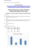
b.

Bar Chart of Grade Frequency
100

75


120

50

25

100
80
60

40

20
0
A

B

C

D

LO02-01

2-1
Copyright © 2015 McGraw-Hill Education. All rights reserved. No reproduction or distribution without the prior written consent of McGraw-Hill
Education.


Chapter 02 - Descriptive Statistics: Tabular and Graphical Method

2.5

a.

(100/250) • 360 degrees = 144 degrees for response (a)

b.

(25/250) • 360 degrees = 36 degrees for response (b)

c.

Pie Chart of Question Response Frequency
D, 50
A, 100

C, 75
B, 25

LO02-01
2.6 a. Relative frequency for product x is 1 – (0.15 + 0.36 + 0.28) = 0.21
b. Product:
N = 0.15 • 500 = 75

W
105

X
Y
180 140

Z

frequency = relative frequency •

c.

54

d.
Degrees for W would be 0.15 • 360 =
for X 75.6
for Y 129.6 for
Z 100.8.
LO02-01

Copyright © 2015 McGraw-

-Hill
Education.


2-2
Hill Education. All rights reserved. No reproduction or distribution without the prior written consent of McGraw


Chapter 02 -

Descriptive Statistics: Tabular and Graphical Method

2.7 a. Rating

Frequency

∑ = 30

Relative Frequency
14

/30 = 0.467
Outstanding
Very Good
Good
Average
Poor

14
10 5
1
0

10

b.

/30 = 0.333
5

/30 = 0.167
1

/30 = 0.033
0

/30 = 0.000

Percent Frequency For Restaurant Rating
50%

47%

40%
33%
30%
20%

17%

10%

3%

0%

Outstanding Very Good

Good

Average

0%
Poor

c.

Pie Chart For Restaurant Rating
Average, 3%

Poor, 0%

Good,
17%

Very Good,
33%

Outstanding,
47%

LO02-01

2-3
Copyright © 2015 McGraw-

-Hill
Education.


Chapter 02 - Descriptive Statistics: Tabular and Graphical Method

Hill Education. All rights reserved. No reproduction or distribution without the prior written consent of McGraw

2.8

a.

Frequency Distribution for Sports League Preference
Sports League

Frequency

Percent Frequency

Percent

MLB

11

0.22

22%

MLS

3

0.06

6%

NBA

8

0.16

16%

NFL

23

0.46

46%

NHL

5

0.10

10%

50

Frequency Histogram of Sports League Preference
25

23

20
15
11
10

8
5

5

3

0
MLB

MLS

NBA

NFL

NHL

b.
c.

Copyright © 2015 McGraw-

-Hill
Education.


Chapter 02 - Descriptive Statistics: Tabular and Graphical Method

Frequency Pie Chart of Sports League Preference
NHL N = 50, 0
NHL 5,
0.1
MLB 11, 0.22
MLS 3, 0.06
NFL 23, 0.46
NBA 8, 0.16

d.

The most popular league is NFL and the least popular is MLS.

LO02-011

2-4
Hill Education. All rights reserved. No reproduction or distribution without the prior written consent of McGraw

2.9

Copyright © 2015 McGraw-

-Hill
Education.

Chapter 02 - Descriptive Statistics: Tabular and Graphical Method

US Market Share in 2005
30.0%

28.3%

26.3%
25.0%
20.0%

18.3%
13.6%

15.0%

13.5%

10.0%
5.0%
0.0%
Chrysler Dodge
Jeep

Ford

GM

Japanese

Other

US Market Share in 2005
Chrysler Dodge
Jeep, 13.6%
Other,
13.5%

Ford, 18.3%
Japanese, 28.3%

GM, 26.3%

LO02-01
2.10 Comparing the pie chart above and the chart for 2010 in the text book shows that between 2005 and
2010, the three U.S. manufacturers, Chrysler, Ford and GM have all lost market share, while
Japanese and other imported models have increased market share.
LO02-01

Copyright © 2015 McGraw-

-Hill
Education.


Chapter 02 - Descriptive Statistics: Tabular and Graphical Method

2-5

Hill Education. All rights reserved. No reproduction or distribution without the prior written consent of McGraw

100%

87%

90%

80%

70%
50%

60%
50%

40%

33%

30%
17%
9%
4%

20%
10%

0%
Private

Mcaid/Mcare No Insurance

Copyright © 2015 McGraw-

-Hill
Education.


Chapter 02 - Descriptive Statistics: Tabular and Graphical Method

2.11 Comparing Types of Health Insurance Coverage Based on Income Level

Copyright © 2015 McGraw-

-Hill
Education.


Chapter 02 - Descriptive Statistics: Tabular and Graphical Method

LO02-01

2-6
Hill Education. All rights reserved. No reproduction or distribution without the prior written consent of McGraw

Copyright © 2015 McGraw-

-Hill
Education.

Chapter 02 - Descriptive Statistics: Tabular and Graphical Method

2.12 a.

Percent of calls that are require investigation or help = 28.12% + 4.17% = 32.29%

b.

Percent of calls that represent a new problem = 4.17%

c.

Only 4% of the calls represent a new problem to all of technical support, but one-third of the
problems require the technician to determine which of several previously known problems
this is and which solutions to apply. It appears that increasing training or improving the
documentation of known problems and solutions will help.

LO02-02

§2.2 CONCEPTS
2.13

a. We construct a frequency distribution and a histogram for a data set so we can gain some insight
into the shape, center, and spread of the data along with whether or not outliers exist.
b.

A frequency histogram represents the frequencies for the classes using bars while in a

frequency polygon the frequencies are represented by plotted points connected by
line segments.

c.

A frequency ogive represents a cumulative distribution while the frequency polygon
does not represent a cumulative distribution. Also, in a frequency ogive, the points
are plotted at the upper class boundaries; in a frequency polygon, the points are
plotted at the class midpoints.

LO02-03
2.14

a. To find the frequency for a class, you simply count how many of the observations have values
that are greater than or equal to the lower boundary and less than the upper boundary.
b.

Once you determine the frequency for a class, the relative frequency is obtained by dividing
the class frequency by the total number of observations (data points).

c.

The percent frequency for a class is calculated by multiplying the relative frequency by 100.
LO02-03

2-7
-Hill Education. All rights reserved. No reproduction or distribution without the prior written consent of McGraw

2.15 a.

Symmetrical and mound shaped:
One hump in the middle; left side is a mirror image of the right side.

Copyright © 2015 McGraw

-Hill
Education.


Chapter 02 - Descriptive Statistics: Tabular and Graphical Method

Double peaked:
b.
the left of which may or may not look
one, nor is each
required to be symmetrical

Two humps,
like the right
hump

c.

Skewed to the Right:
Long tail to the right

Skewed to the left:
d.
tail to the left

Long

LO02-03

Descriptive Statistics: Tabular and
Method

Graphical

§2.2 METHODS AND APPLICATIONS
2.16 a.

Since there are 28 points we use 5 classes (from Table 2.5).

b.

Class Length (CL) = (largest measurement – smallest measurement) / #classes = (46 – 17) / 5 = 6
(If necessary, round up to the same level of precision as the data itself.)

c.

The first class’s lower boundary is the smallest measurement, 17.
The first class’s upper boundary is the lower boundary plus the Class Length, 17 + 3 =

2-8
Copyright © 2015 McGraw-Hill Education. All rights reserved. No reproduction or distribution without the prior written consent of McGraw-Hill
Education.


Chapter 02 -

23 The second class’s lower boundary is the first class’s upper boundary, 23
Continue adding the Class Length (width) to lower boundaries to obtain the 5
classes: 17 ≤ x < 23 | 23 ≤ x < 29 | 29 ≤ x < 35 | 35 ≤ x < 41 | 41 ≤ x ≤ 47
d.

Frequency Distribution for Values
lower
17
23
29
35
41

upper

midpoint

< 23
< 29
< 35
< 41
< 47

20
26
32
38
44

width

cumulative

cumulative

frequency

percent

frequency

percent

4
2
4
14
4
28

14.3
7.1
14.3
50.0
14.3
100.0

4
6

10
24
28

14.3
21.4
35.7
85.7
100.0

6
6
6
6
6

e.

f.

See output in answer to d.

LO02-03

Copyright © 2015 McGraw

2.17 a. and b. Frequency Distribution for Exam Scores
2-9
-Hill Education. All rights reserved. No reproduction or distribution without the prior written consent of McGraw-Hill
Education.

Chapter 02 - Descriptive Statistics: Tabular and Graphical Method

relative
lower

upper

midpoint

width

frequency

percent frequency

cumulative

cumulative

frequency

percent

50

< 60

55

10

2

4.0

0.04

2

4.0

60

< 70

65

10

5

10.0

0.10

7

14.0

70

< 80

75

10

14

28.0

0.28

21

42.0

80

< 90

85

10

17

34.0

0.34

38

76.0

90

< 100

95

10

12

24.0

0.24

50

100.0

50

100.0

c.

Frequency Polygon
40.0
35.0
30.0
25.0
20.0
15.0
10.0

5.0
0.0
4
0

50

60

70

80

90

Data

d.
Ogive
100.0

75.0

50.0

25.0

0.0
40

50

60

70

80

90

Data

2-10
Copyright © 2015 McGraw-Hill Education. All rights reserved. No reproduction or distribution without the prior written consent of McGraw-Hill
Education.


Chapter 02 -

LO02-03

2-11
-Hill Education. All rights reserved. No reproduction or distribution without the prior written consent of McGraw-Hill
Education.


Chapter 02 -

a.
Descriptive Statistics: Tabular and Graphical Method

2.18

Because there are 60 data points of design ratings, we use six classes (from Table 2.5).

b.

Class Length (CL) = (Max – Min)/#Classes = (35 – 20) / 6 = 2.5 and we round up to 3, the
level of precision of the data.

c.

The first class’s lower boundary is the smallest measurement, 20.
The first class’s upper boundary is the lower boundary plus the Class Length, 20 + 3 =
23 The second class’s lower boundary is the first class’s upper boundary, 23
Continue adding the Class Length (width) to lower boundaries to obtain the 6 classes:
| 20 < 23 | 23 < 26 | 26 < 29 | 29 < 32 | 32 < 35 | 35 < 38 |

d.

Frequency Distribution for Bottle Design Ratings

lower
20
23
26
29
32
35

e.

upper
<
<
<
<
<
<

23
26
29
32
35
38

cumulative

cumulative

midpoint

width

frequency

percent

frequency

percent

21.5
24.5
27.5
30.5
33.5
36.5

3
3
3
3
3
3

2
3
9
19
26

1
60

3.3
5
15
31.7
43.3
1.7
100

2
5
14
33
59
60

3.3
8.3
23.3
55
98.3
100

Distribution shape is skewed left.

Copyright © 2015 McGraw-

-Hill

Education.


Chapter 02 - Descriptive Statistics: Tabular and Graphical Method

a.

LO02-03

2-11
Hill Education. All rights reserved. No reproduction or distribution without the prior written consent of McGraw

2.19 a & b. Frequency Distribution for Ratings
relative
lower
20
23
26
29
32
35

upper midpoint
<
<
<
<
<
<

23
26
29
32
35
38

21.5
24.5
27.5
30.5
33.5
36.5

cumulative relative

cumulative

width

frequency

percent

frequency

percent

3
3

3
3
3
3

0.033
0.050
0.150
0.317
0.433
0.017
1.000

3.3
5.0
15.0
31.7
43.3
1.7
100

0.033
0.083
0.233
0.550
0.983
1.000

3.3
8.3

23.3
55.0
98.3
100.0

c.

2-13
Copyright © 2015 McGraw-Hill Education. All rights reserved. No reproduction or distribution without the prior written consent of McGraw-Hill
Education.


Chapter 02 - Descriptive Statistics: Tabular and Graphical Method

Ogive
100.0

75.0

50.0

25.0

0.0
17

20

23

26

29

32

35

Rating

LO02-03
2.20 a.
2.5).

Because we have the annual pay of 25 celebrities, we use five classes (from Table

Class Length (CL) = (290 – 28) / 5 = 52.4 and we round up to 53 since the data are in whole
numbers.
The first class’s lower boundary is the smallest measurement, 28.
The first class’s upper boundary is the lower boundary plus the Class Length, 28 + 53 = 81
The second class’s lower boundary is the first class’s upper boundary, 81
Continue adding the Class Length (width) to lower boundaries to obtain the 5 classes:
| 28 < 81 | 81 < 134 | 134 < 187 | 187 < 240 | 240 < 293 |

2-12
Hill Education. All rights reserved. No reproduction or distribution without the prior written consent of McGraw

2.20

(cont.)

Frequency Distribution for Celebrity Annual Pay($mil)
lower
28

< upper
< 81

midpoint
54.5

width
53

frequency
17

Copyright © 2015 McGraw-

percent
34.0

cumulative

cumulative

frequency
17

percent

34.0

-Hill
Education.


Chapter 02 - Descriptive Statistics: Tabular and Graphical Method

a.
81
134
187
240

<
<
<
<

134
187
240
293

107.5
160.5
213.5
266.5

53

53
53
53

6
0
1
1
25

12.0
0.0
2.0
2.0
50.0

23
23
24
25

46.0
46.0
48.0
50.0

Histogram of Pay ($mil)
18
16
14

12
10
8
6
4
2

c.

0

28

81

134

187

240

293

Pay ($mil)

Ogive
100.0

75.0

50.0

25.0

0.0
28

81

134
187
Pay ($mil)

240

LO02-03

2-15
Copyright © 2015 McGraw-Hill Education. All rights reserved. No reproduction or distribution without the prior written consent of McGraw-Hill
Education.


Chapter 02 - Descriptive Statistics: Tabular and Graphical Method

a.
2.21

The video game satisfaction ratings are concentrated between 40 and 46.
b.

Shape of distribution is slightly skewed left. Recall that these ratings have a minimum value
of 7 and a maximum value of 49. This shows that the responses from this survey are
reaching
near to the upper limit but significantly diminishing on the low side.

c.

Class:

1

Ratings:
d.

2

3

4

341
4
13
25

Cum Freq:

5
40

45

6

7

4261
65

LO02-03
2.22 a.

The bank wait times are concentrated between 4 and 7 minutes.

b.

The shape of distribution is slightly skewed right. Waiting time has a lower limit of 0 and
stretches out to the high side where there are a few people who have to wait longer.

c.

The class length is 1 minute.

d.

Frequency Distribution for Bank Wait Times

lower
-0.5

0.5
1.5
2.5
3.5
4.5
5.5
6.5
7.5
8.5
9.5
10.5
11.5

<
<
<
<
<
<
<
<
<
<
<
<
<
<

upper
0.5

1.5
2.5
3.5
4.5
5.5
6.5
7.5
8.5
9.5
10.5
11.5
12.5

midpoint
0
1
2
3
4
5
6
7
8
9
10
11
12

width
1

1
1
1
1
1
1
1
1
1
1
1
1

frequency
1
4
7
8
17
16
14
12
8
6
4
2
1
100

percent

1%
4%
7%
8%
17%
16%
14%
12%
8%
6%
4%
2%
1%

cumulative

cumulative

frequency
1
5
12
20
37
53
67
79
87
93
97

99
100

percent
1%
5%
12%
20%
37%
53%
67%
79%
87%
93%
97%
99%
100%

LO02-03

Copyright © 2015 McGraw-

-Hill
Education.


Chapter 02 - Descriptive Statistics: Tabular and Graphical Method

a.
2-14

Hill Education. All rights reserved. No reproduction or distribution without the prior written consent of McGraw

2.2
3
The
tras
h
bag
brea
kin
g
stre
ngt
hs
are
con
cent
rate
d
bet
wee

n 48 and 53 pounds.
b.

The shape of distribution is symmetric and bell shaped.

c.

The class length is 1 pound.

d.

Class:
46<47 47<48 48<49 49<50 50<51 51<52 52<53 53<54 54<55
Cum Freq. 2.5% 5.0%
15.0% 35.0% 60.0% 80.0% 90.0% 97.5% 100.0%
Ogive
100.0

75.0

50.0

25.0

3.3
100.0

30

0.0
45

47

49

51

53

Strength

Histogram of Value $mil
25

20

15

10

5

0
304

584

864
1144
Value $mil

1424

1704

LO02-03
2.24 a.

Because there are 30 data points, we will use 5 classes (Table 2.5). The class length will be
(1700-304)/5= 279.2, rounded to the same level of precision as the data, 280.
Frequency Distribution for MLB Team Value ($mil)

lower upper midpoint
304 < 584
percent
1424 < 1704 584 < 864
1564 864 < 1144
280 1144 < 1424
1

30

width
444
724
1004
1284

cumulative
cumulative
frequency
percent frequency
280
24
80.0
24
280

4
13.3
28
280
1
3.3
29
280
0
0.0
29

80.0
93.3
96.7
96.7

100.0

2-17
Copyright © 2015 McGraw-Hill Education. All rights reserved. No reproduction or distribution without the prior written consent of McGraw-Hill
Education.


- Descriptive Statistics: Tabular and Graphical Method

Distribution is skewed right and has a distinct outlier, the NY Yankees.
Chapter 02

2.24 b.

Frequency Distribution for MLB Team Revenue
upper midpoint
143 < 200
171.5
200 < 257
228.5
257 < 314
285.5
314 < 371
342.5

width
57
57
57
57

cumulative
cumulative lower
frequency
percent frequency
percent
16
53.3
16
53.3
11
36.7
27

90.0
2
6.7
29
96.7
0
0.0
29
96.7

Copyright © 2015 McGraw-

-Hill
Education.


Chapter 02 - Descriptive Statistics: Tabular and Graphical Method

a.
3.3
100.0

30
Histogram of Revenues $mil
18
16
14
12
10

8
6
4
2
0

143

200

257

314

Revenues $mil

371

428

The distribution is skewed right.
c.
Percent Frequency Polygon
100.0

80.0
60.0
40.0
20.0
0.0

304

584

< 428

399.5

864
1,144 1,424
Value ($mil)

LO02-03
371

57

1

30

100.0

2-19
Copyright © 2015 McGraw-Hill Education. All rights reserved. No reproduction or distribution without the prior written consent of McGrawHill Education.