A practical guide to RF and mixed signal printed circuit board layout

Contents
Table of Figures
List Of Tables
Acknowledgements.
Forward
So What’s The Difference Between Analog And Digital?
Do We Still Use Analog?
What’s The Frequency?
When Does Analog Become RF?
Converging Domains
Analog / RF Issues To Consider
Loss
Dielectric Loss
Skin Effect
Return Loss Or VSWR
Noise / Coupling / EMI / Shielding
Clean Power Delivery
A Few things Before Starting The Design
The Schematic And Mechanical Drawings
The Circuit Blocks
Slots And Splits In Power And Ground Planes
High speed return current
Fringe fields
Some exceptions
Power planes
Isolate In X/Y Axis
Isolate In Z Axis
Isolate In X/Y Axis And Z Axis

Layer 2 And Layer 3 Usage
Choosing Between Single And Dual Stripline
Useful RF And Mixed Technology Stackups
4 Layer RF Only Design Stackup
6 Layer RF Only Design Stackup
8 Layer XYZ Mixed RF - Digital Design Stackup – Low Density Digital
10 Layer Mixed RF - Digital Design Stackup – Low To Medium Density Digital
12 Layer Mixed RF - Digital Design Stackup – Medium To High Density Digital
14 Layer Mixed RF - Digital Design Stackup – High Density Digital
16 Layer Mixed RF - Digital Design Stackup – High Density Digital
It’s A Material World
On The Right Wavelength ?
Processes And Cost
Transmission Lines
Dispersion
Microstrip
Structure
Impedance Calculation
Advantages
Disadvantages
Embedded Microstrip
Structure
Impedance Calculation
Advantages
Disadvantages
Stripline
Structure
Impedance Calculation
Advantages
Disadvantages

Coplanar Waveguide (CPW)
Structure
Impedance Calculation
Notes:
Advantages
Disadvantages
Component Selection
A Place For Everything
The Long And The Short Of It
Power Delivery, Decoupling and Bypassing
Decoupling
Bypassing
Bypassing Low Frequency Analog Circuits
Bypassing RF Circuits
Bypassing Digital Circuits
Capacitor Selection
Placing And Routing Decoupling And Bypass Capacitors
Routing Mixed Technology Printed Circuit Boards
Net Classes And Constraints
Classes
Constraints
Routing
Do Not Route Signals Over Splits In Reference Planes
No Vias In RF Or High Speed Digital Signal Paths
No Stubs Allowed In Signal Path Routing
Traces, Shapes And Modified Footprints
Corners In RF Traces
T-Junctions And Power Dividers In RF Traces

Matching Transmission Line Width To Pad Geometries
Ground: Copper Floods, Vias and Shielding


Flooding Unused Areas With Ground
Adding Ground Vias
Ground Shielding Vias
Ground Stitching Vias
Ground Transition Vias
EMI Shielding Vias
Shielding
Summary
Conclusion


Table of Figures
Figure 1. Cross Section Of Current Flow At low And High Frequencies Showing Skin Effect.
Figure 2. Voltage Reflection Where Load Impedance Is Higher Than Line Impedance.
Figure 3. Voltage Reflection Where Load Impedance Is Lower Than Line Impedance.
Figure 4. Power Implemented As A Wide Trace.
Figure 5. Power Implemented As A Local Plane - Potential Patch Antenna.
Figure 6. Example Of When An Impedance Mismatch Becomes An Issue - @ f = 5GHz
Figure 7. Floorplan View Of X/Y Axis RF And Digital Zone Isolation.
Figure 8. Cross Section View X/Y Axis Only RF And Digital Zone Isolation.
Figure 9. Z Axis Isolation Of RF And Digital Circuitry.
Figure 10. Floorplan View X/Y And Z Axis RF And Digital Zone Isolation.
Figure 11. Cross Section View X/Y And Z Axis RF And Digital Zone Isolation.
Figure 12. Layer 3 As Reference Ground For Microstrip Allows Wider Transmission Line.
Figure 13. Difference Between Past And Present Typical Digital Routing.
Figure 14. Typical 4 Layer RF Only Stackup Cross Section.

Figure 15. Typical 6 Layer RF Only Stackup Cross Section.
Figure 16. Typical 8 Layer Mixed RF/Digital Stackup Cross Section.
Figure 17. Typical 10 Layer Mixed RF/Digital Stackup Cross Section.
Figure 18. Typical 12 Layer Mixed RF/Digital Stackup Cross Section.
Figure 19. Typical 14 Layer Mixed RF/Digital Stackup Cross Section.
Figure 20. Typical 16 Layer Mixed RF/Digital Stackup Cross Section.
Figure 21. Differences In Fiber Density With Different Weave Styles.
Figure 22. Advantages And Examples Of Via In Pad Technology.
Figure 23. Resistive Model Of A DC Or Low Speed Transmission Line.
Figure 24. Complete Model Of A High Speed Transmission Line Showing Parasitic Elements.
Figure 25. Microstrip Transmission Line Construction.
Figure 26. Embedded Microstrip Transmission Line Construction.
Figure 27. Stripline Transmission Line Construction.


Figure 28. Coplanar Waveguide Transmission Line Construction.
Figure 29. Example Of Keeping Input And Output Of A Circuit Block Well Distanced.
Figure 30. Amplifier And Filter With Overlapping Loop Areas.
Figure 31. Modified Amplifier Bypassing To Reduce Loop Area.
Figure 32. Floorplan Of Typical RF Modem Design With Baseband Processing And Power
Supplies.
Figure 33. Noise Transients Can Travel Anywhere On The Board.
Figure 34. Well Selected And Placed Decoupling Capacitors Can Keep Power Planes Much
Cleaner.
Figure 35. Bypass Capacitors On Analog Device Can Remove Noise Already Existing On Power
Connections.
Figure 36. Bypass Network Frequency Response With All Low ESR Capacitors.
Figure 37. Bypass Network Frequency Response May Improve If One Or More Capacitors Have
Higher ESR.
Figure 38. General Placement Of Discrete Parts Around Large Integrated Devices.

Figure 39. Placement And Via Usage For BGA Bypassing.
Figure 40. Placement And Connections For Bypassing QFP With Thermal Pad.
Figure 41. Placement And Connections For Bypassing QFP Without Thermal Pad.
Figure 42. Connections To Power Plane For Decoupling Capacitors Around High Density Digital
Devices.
Figure 43. Connections To Plane With Bypass Capacitors ‘On The Way’ For An Analog Amplifier.
Figure 44. Slot In Ground Plane Causes Long Ground Return Path.
Figure 45. Example Placement With Resulting Return Paths And Loop Areas.
Figure 46. Adding A Ground Plane Split To Restrict Ground Current Paths.
Figure 47. Stub Caused By A Through Via Being Accessed On An Internal Layer.
Figure 48. Back-drill Eliminates Most Of The Stub, Blind Via Or Microvia Eliminates The Stub.
Figure 49. Routing The Same Connection With And Without Stubs.
Figure 50. Improved Placement And Via-In-Pad Technology Can Easily Remove Stubs In RF Design.
Figure 51. Offset Pad Origin Can Resolve DRC Errors On Small Components.
Figure 52. Footprint Based Rule Area Can Resolve DRC Errors On Small Components.
Figure 53. Tapered Transitions To Transmission Line Width Can Be Built Into The Footprints.


Figure 54. The 90 Degree Corner - Worst Case Method And Best Case Method.
Figure 55. Different Ways To Implement 90 Degree Bends in RF Transmission Lines.
Figure 56. Impedance Mismatch Area With Simple T-Junction.
Figure 57. T-Junction Impedance Mismatch And Commonly Used Compensations.
Figure 58. Transmission Line Geometry Does Not Match Component Pad Geometry.
Figure 59. Removing Planes Copper Beneath Large Component Pads.
Figure 60. Stepped And Tapered Matching Of Transmission Line To Pad Geometry.
Figure 61. Ground Stitching Along RF Signal Paths - Maintain 3H Spacing To Traces.
Figure 62. Ground Stitching Along RF Traces And Under Perimeter Shield Walls.
Figure 63. Ground Stitching Vias Added Where Space Permits Around The Design.
Figure 64. Effect On Ground Return Current If There Are No Ground Vias Nearby
Figure 65. Ground Vias And Antipad At Differential Pair Layer Transition.

Figure 66. Some Typical Perimeter EMI Shielding Via Patterns.
Figure 67. An Example Of Standard Off The Shelf Shielding Products.
Figure 68. Photo Etched Shielding Can Be Custom Shaped And More Complex.
Figure 69. Some Examples Of Custom Milled RF Enclosures.


List Of Tables
Table 1. Common Circuit Board Materials Of Different Compositions With Loss And Dielectric
Constant.
Table 2. Suggested Layer Usage For Typical 4 Layer RF Only Stackup.
Table 3. Suggested Layer Usage For Typical 6 Layer RF Only Stackup.
Table 4. Suggested Layer Usage For Typical 8 Layer Mixed Technology Stackup.
Table 5. Suggested Layer Usage For Typical 10 Layer Mixed Technology Stackup.
Table 6. Suggested Layer Usage For Typical 12 Layer Mixed Technology Stackup.
Table 7. Suggested Layer Usage For Typical 14 Layer Mixed Technology Stackup.
Table 8. Suggested Layer Usage For Typical 16 Layer Mixed Technology Stackup.
Table 9. Difference In Signal Wavelength In Air And In Different Circuit Board Environments.
Table 10. Typical SMD Bypass Capacitors And Their Useful Frequency Ranges.


Acknowledgements
The author would like to express thanks and appreciation to the following people, without whom it
would not have been possible to put this guideline together.
Nick Barbin. President - Optimum Design Associates. For providing the idea, encouragement,
patience, and the time to compile and present the guideline. This guideline took many hours to
produce and would not have been possible if the time was not proved to do so.
Scott Nance. Senior Designer - Optimum Design Associates. For his invaluable assistance in so many
ways. Scott spent many hours reading word by word, providing extremely useful content, corrections,
feedback and suggestions for improvement. Scott has also presented this guideline in slide
show/discussion form at trade shows and at specific customer sites.

Rick Hartley. Industry recognized consultant on the topic of High Speed and Mixed Technology
Design. Rick was kind enough to volunteer his time to read the guideline completely and provided
much extremely useful feedback and some very critical and needed corrections to the content.
Robert Frank. Marketing Manager - Optimum Design Associates. For many hours of proof-reading,
grammar correction and for getting this book published.
Optimum Design Associates Designers. The entire design group at Optimum Design Associates.
These include Randy Holt, Scott Nance, Juliet Wang, Tom Stout, Mark Gutierrez, Frank Jacobson,
Brian Noble, Rick Dachauer. All of these designers have contributed over the years by way of being
part of a collaborative team of senior designers. We all have both common and specific skills and
learn from each other.


Forward
This guideline is presented as a practical guide to the physical layout design of RF and, in particular,
mixed technology circuit boards. Mixed technology refers to the combination of low frequency
analog, high frequency RF, power supplies, digital circuitry and even motor drivers, all in a single
design. The guideline does not present pages of RF theory and formulae, those are for the electrical
engineer and the engineering design has already been done by the time the circuit board layout
process is started. Some formulae and theory are presented however, not for the day to day design
process but more as an aid to understanding some of the things layout designers need to consider more
for mixed technology design than would be the case in a purely digital design. One of the main aims
of this guideline is to use plain words wherever possible to present information that is normally
presented with a lot of formulae, numbers and theory and which is, quite frankly, lost on most layout
designers. What the layout designer needs is information on what to do at the circuit board level when
designing the physical layout, not the engineering circuit. The circuit board layout process is the last
real design phase in the product development cycle, and it is certainly the phase that is normally
placed under the most pressure in terms of time to complete, because everything that comes before it
always takes longer than the time budgeted. As a result, the layout designer needs to be as efficient as
possible and make use of proven methods and techniques to complete the task in as timely a manner
as possible while still being technically correct. The issues faced when designing circuit boards for

RF and mixed technology applications that are not usually considered so critically in designs for only
digital applications will be described. Techniques and methods will be presented that have been used
consistently over many years of designing circuit boards for all types of applications, many of which
were for radar systems, RF modems and satellite payload systems.
Some of these methods and techniques may be considered technically unnecessary or may well
conflict with what some designers currently do or are advised to do by their peers, but everything
presented in this guideline has been used very successfully over a long period of time designing
mixed technology circuit boards. There is no ‘one size fits all’ solution to the challenge of mixed
technology design. There are many different views and approaches to the problem. Electrical
engineers, layout designers, actual designs, constraints and CAD tools each differ greatly and yet we
are still able to produce designs that work well despite all these variations, so there are clearly many
methods that do work well. Although this guideline is much more for layout designers rather than the
electrical engineers, there is also much useful information for electrical engineers which will help
them to understand some of the real world design, fabrication and assembly issues that layout
designers face in the process of producing the layout and that they themselves would rarely consider.


So What’s The Difference Between Analog And
Digital?
Understanding the main differences between these two design types is a key part of understanding
why some things the layout designer does will have a more significant effect in one design type versus
the other. In truth, the more challenging design is still the analog one, because the big difference is that
in analog design some things need to be considered a lot more carefully than they would be when
doing a purely digital design. A layout designer still needs to consider the same things in digital
design, but often to a significantly lesser degree because digital designs can be reasonably tolerant to
many of these issues. Having said that, as operating frequencies increase and logic voltage levels
decrease in digital circuits, layout designers are finding that issues traditionally more important in
analog circuits are becoming just as important in digital circuit layouts. The differences between
digital and analog domains are, with respect to circuit board layout, becoming less and less obvious.

Information Integrity.
Just as in a digital design, the critical issue in an analog design can be thought of as being ‘information integrity’. In a digital
design the information is being conveyed by means of ‘ones and zeros’, the circuits generate and respond to discrete voltage
levels representing a binary 1 or 0. Typically a high voltage represents a 1, and a low or zero voltage represents a 0. There is
usually no information conveyed by voltage levels other than those. In an analog design, information is conveyed, in different
ways, by voltage levels continuously variable from microvolts to tens or even hundreds of volts. Similarly, the frequency in a
digital system, with few exceptions, simply controls how fast the data is conveyed or processed, while in an analog system the
frequency of a signal often IS the information content of the signal. The phase of an analog signal and its relationship to the
phase of another signal is often the information content of an analog system as well.

Amplitude, frequency and phase are also extremely important in a digital design, but digital systems
are usually more tolerant to some degradation in all of these, some to a lesser extent than others.
However, in an analog system, there can be very little tolerance to degradation in any of these
parameters because they ARE the information being processed.
Placement and routing of RF circuits is far more critical than with digital circuits. Placement is
critical because inputs and outputs need to be physically separated, discrete component placement
(especially inductive components) is very critical and the circuit needs to ‘flow’ in a sensible
manner. The main criterion for digital circuit placement is usually easiest routing before anything
else. Even though there are far fewer signals involved, routing is also more critical in RF designs
because the copper connections, while performing the normal connectivity function of a trace, are
also now functional circuit elements in their own right. Traces and component pads have resistive,
capacitive and inductive properties. At extremely high frequencies these trace and pad properties
contribute significantly to the overall circuit behavior. All metal on an RF circuit board should be
considered RF-functional.


Do We Still Use Analog?
While we may be living in the digital age, analog circuits are still prevalent, and we use them every
day. Equipment with significant analog circuit content includes things like cell phones, audio
amplifiers, instrumentation amplifiers, radio receivers, data acquisition and measurement circuits,

medical imaging, monitoring and treatment equipment, power supplies and, of course, RF and
microwave circuits used in satellite and radar systems. Most equipment using analog circuits today
also includes some digital circuitry. For example, an audio amplifier/receiver contains a lot of
sensitive and critical analog circuitry for audio processing, both at extremely low levels at the inputs
and very high levels at the outputs. It also contains increasing amounts of digital circuitry for such
functions as digital tuning, volume and tone controls, analog to digital conversion and processing to
add predefined effects to the sounds and then conversion back to analog for output to the speakers.
There is also storage and retrieval of the analog data on digital media because it is far more reliable,
portable, lower cost and much faster than analog storage media like disc records and tapes.


What’s The Frequency?
With analog and RF systems, signals tend to consist of a single or small number of fundamental
frequencies. There are usually multiple signals of interest, but it is a smaller number of different
frequencies or a specific range of frequencies that the layout designer is concerned with. All other
frequencies present would be considered as noise or interference signals which need to be controlled
or filtered out so that only the frequencies of interest are processed as effectively as possible. There
will, of course, be some harmonics of these intended frequencies present but typical RF designs
utilize many filters in the signal path to ensure that only signals of the frequencies of interest are
passed to or from circuit blocks. In digital designs, signals are what we call square waves. A square
wave is actually the sum of a sine wave of the same (fundamental) frequency, plus all the odd
harmonics of that frequency at diminishing amplitudes. A faster rise time of a digital signal indicates
that there are more high frequency harmonics present. So in any digital system you will have signals
present of much higher frequency that you might think. Hence the term ‘it’s not the frequency that
matters, it’s the edge rate’, because a faster edge rate (rise time) indicates the presence of much
higher frequency content than the actual ‘clock frequency’. Many layout designers simply look at the
clock frequency and think that this is the frequency that they are ‘designing for’ when, in reality, there
are much higher frequencies present that should be considered.

When Does Analog Become RF?
Traditionally, analog circuits were low frequency systems for supply of power and for voice and
audio signal processing, because that’s what we developed electronics for first – the telephone for
example. RF circuits were developed for long distance real time communication, where we could
now transmit our voices over long distance through Radio Frequency waves rather than having to
have a solid wire between two or more points. These systems produced, transmitted and received
radio frequency signals ranging from hundreds of KHz to hundreds of MHz.

It has become normal to think of RF as being in the 3 MHz – 300 MHz range. Analog circuits
operating in the 300 MHz – 300 GHz range were traditionally referred to as microwave circuits.
There are many opinions on when an RF signal becomes microwave, with above 300 MHz is the
generally accepted point. Between 30 GHz and 300 GHz is often referred to as Millimeter Wave
because the wavelength in this band ranges from 10mm to 1mm, but generally microwave refers to
everything above 300 MHz.

Given these frequency ranges, it is clear that most digital circuits today are operating well into what
are traditionally known as the RF and microwave frequency ranges. In this guideline we do not focus
on the difference between frequency ranges, but more on what a layout designer can do to help these
fundamentally different circuit types operate in harmony together on a single circuit board and at a
wide range of frequencies.


Converging Domains
Much of what is presented in this guideline will use terms most layout designers have already heard
in reference to digital designs. Impedance matching, transmission lines, return loss, coupling, noise
and interference, crosstalk, delay tuning, signal integrity etc. are all terms layout designers have
become familiar with over the last decades. That is because these are predominantly high frequency
related terms describing phenomena that layout designers need to be aware of, and are becoming
more prevalent because digital designs are operating at higher and higher frequencies all the time.
Well, it is not new terminology by any means. These are things that have been the concern of RF and

analog electrical engineers and layout designers for the last 50 years or more. In the early days of
digital systems, voltage levels were 5 Volts, 10 Volts or even higher. Frequencies were in the
hundreds of KHz and very low MHz ranges with much longer rise times than is the case today. At
these low frequencies, and with these voltage levels (the voltage levels required to cause a change
from a 0 to a 1 were in the order of 3 volts or more) there was an inherent immunity to noise virtually
built in. There was much less noise to consider anyway, because such slow circuits did not cause
much significant radiation. Today, some digital circuits are operating at sub 1 Volt levels, with the
logic thresholds diving into the hundreds of millivolts range, and with frequencies into the GHz
ranges with sub-nanosecond edge rates, so the high frequency content and EMI radiation are much
increased. Today’s high speed digital designs really do need to be treated as low level high
frequency analog designs.


Analog / RF Issues To Consider


Loss
One of the primary concerns in analog and RF systems is the efficient transfer of power. All of the
signal power present at the output of any circuit block should ideally be transferred to the next stage
of the circuit. When a signal needs to be attenuated, it should be done in a controlled manner using an
attenuator device that will produce predictable and repeatable results. Signal power losses due to
non-circuit elements like impedance mismatch, incorrect transmission line design or material
selection issues are potentially detrimental to the functioning of the circuit. Some losses are
unavoidable, there is no such thing as a perfect signal environment. There are losses inherent in the
circuit board materials and there are losses as a result of design parameters and techniques.


Dielectric Loss
Dielectric loss, specified as dissipation factor (Df) on a vendor’s datasheet, (which will never be
zero), is inherent in the laminate and prepreg materials used to fabricate the board. It is the loss of

energy that goes to heating a dielectric material in a changing electromagnetic field and, in circuit
board laminates, is a function of the materials’ molecular structure and resin type and content. There
are a very wide range of materials available, some of which exhibit dielectric loss orders of
magnitude lower than others. Dielectric loss is proportional to frequency, and is therefore more
critical to consider with higher frequency lower power designs.

The following table lists some commonly used printed circuit materials and their corresponding
dielectric loss values.


Material
ISOLA
370HR
ISOLA
FR408HR
NELCO
N4000-13 EP
SI
PANASONIC
MEGTRON 6
ROGERS
RO4350B
NELCO
7000-2 V0
ARLON
CLTE XT
TACONIC
TacLamplus

Composition

Df
Dk
Relative PCB
@10GHz @10GHz Tg cost/Mfg Tier

Epoxy/Woven Glass

0.025

3.92

180 1-FR-4

Epoxy/Woven Glass

0.0095

3.65

190 2-LowLoss

Epoxy/Cyanate Ester/Woven
Glass

0.007

3.2

Epoxy/PPE/Woven Glass

0.004
Hydrocarbon/Ceramic/Woven
Glass
0.0037

3.3

Polyimide/Woven Glass

0.010

3.8

PTFE/Ceramic/Woven Glass

0.0012

2.94

210 2-LowLoss
3185 UltraLowLoss
3280 UltraLowLoss
4250 Performance
4230 Performance

PTFE/Metal Backed

0.0004

2.1

230 5-Custom

3.48

Table 1. Common Circuit Board Materials Of Different Compositions With Loss And Dielectric
Constant.


Formulae and equations can be found that will translate this information into dB loss values at
particular frequencies. That level of detail is not presented here because, as a layout designer, the
main concern is, “What am I contributing to loss?” Dielectric loss is beyond the control of a layout
designer unless the layout designer is also entirely responsible for material selection. Lower loss
materials are more expensive, so, in many cases, they are not even a consideration. The layout
designer needs to be aware of the phenomena and which materials are better for a particular design,
in order to make valid recommendations regarding material selection.

In an analog design, when a signal is injected into a transmission line, the frequency of the propagated
wave will be unchanged, but the amplitude will be decreased due to dielectric loss. The amount of
loss will be dependent on the length of the transmission line, and the frequency of the signal (because
dielectric loss is proportional to frequency). This is one of the reasons we always strive to keep
higher frequency connections as short as possible. Extremely low level analog circuits, such as
instrumentation amplifiers or low power receiver front ends, require consideration of dielectric loss
because of the intolerance of these circuits to amplitude loss.

Digital signals are square waves, which consist of the fundamental frequency plus an infinite number
of embedded sine waves at odd harmonics (odd multiples of the fundamental frequency) and at
diminishing amplitudes. Digital signals generally have very strong amplitude at the fundamental and
lower harmonic frequencies up to an approximate frequency as determined by the equation:

f = 0.35 / Tr
where f = frequency in GHz

and

Tr = Signal Rise Time in nanoseconds.

Digital signals contain a bandwidth of frequencies, from the fundamental frequency to the frequency
determined by the above equation, which are particularly affected by dielectric loss. Most digital
circuits will operate quite well on the ‘standard’, higher loss materials, but material selection must be
considered when digital circuits are operating above 3 - 5 GHz. Evolving device technologies also
means that edge rates are becoming faster, therefore overall frequency content is increasing, even if
the ‘clock frequency’ is kept the same, so it may well be that using a low loss material becomes a
necessary consideration for a design where it may not have normally been considered.


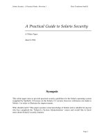
Skin Effect
Conductor loss is related to the way current flows in a conductor. At low frequencies, current in a
conductor will flow in the entire cross section of the conductor. At higher frequencies, current tends
to concentrate in the thin outer portion of the trace. (See Figure 1) This is known as Skin Effect. This
phenomena effectively reduces the cross sectional area of the conduction path, making it more
resistive. This can be offset to a certain extent by using wider traces where impedance modelling
allows. Wider traces will exhibit less variation in resistance with frequency so the trace will be less
lossy. Because it increases the effective resistance of the signal path, skin effect also has an effect on
transmission line impedance, making selection of the correct termination resistor values more
complex.

Smooth surface is better.
Copper surface roughness contributes to increased loss due to skin effect because the overall resistance of the path is a
function of the path length. At higher frequencies, the skin effect causes the current to flow in a much thinner region of the

trace, at or near the surface. The rougher the surface is, the longer and therefore more resistive will be the signal path.

The approximate skin depth of copper is:

Skin Depth (cm) =

or Skin Depth (inch) =

It is also known that there will be considerably more current flow in the surface closest to the
reference plane. So, when designing the stackup, try to make the reference plane the layer above the
trace rather than the layer below the trace. This will concentrate the current in the top of the trace,
which is smoother and therefore shorter. The surface of the copper bonded to the laminate can be
extremely rough, and this makes the signal path a lot longer. Use of rolled copper laminates would
also help to mitigate the loss due to skin effect, because the bonded edge of the copper is smoother.
Many laminate manufacturers are now also offering materials with very much smoother surfaces at the
junction between the copper and the base material in an effort to mitigate the skin affect as much as
possible. Because material selection is often driven by the RF electrical engineer, or by cost factors,
it is something the layout designer does not always control. However, understanding the different
materials and when to utilize them can allow the layout designer to make valuable recommendations.


Figure 1. Cross Section Of Current Flow At low And High Frequencies Showing Skin Effect.


Return Loss Or VSWR
A full discussion of return loss and Voltage Standing Wave Ratio (VSWR) would easily be the
subject of an entire book by itself. A detailed examination would involve a large amount of very
complex mathematics to explain what becomes quite a dynamic issue, when changing signal
frequencies and amplitudes, along with transmission line characteristics, variable source and load
impedances and skin effect are all combined. Such a discussion is beyond the scope of this guideline,

and is actually more in the engineering domain than in the circuit board design domain. Usually the
most significant contributor to loss in an RF design is return loss. This is the loss caused by mismatch
between the output impedance of a driving source, the characteristic impedance of the connecting
transmission line, and the input impedance of the receiving load. This discussion assumes a voltage
source with a purely resistive output impedance providing a single frequency sine wave into a purely
resistive line and load. There are a limited number of things that a layout designer can do to either
cause or help resolve return loss and VSWR issues.

Impedance is a frequency dependent quantity. This means the characteristic impedance of the
transmission line and the source and load impedances will vary with frequency. When a signal travels
along a transmission line and then arrives at the load, if there is a mismatch between the characteristic
impedance of the transmission line and the impedance of the load, then a portion of the signal will be
reflected back along the transmission line towards the source. The polarity and magnitude of the
reflected signal depends on whether the load impedance is higher or lower than the line impedance:
(assume that the source and line impedances are perfectly matched.)

If the load impedance exactly matches the line impedance then there is maximum power transfer to the
load and there is zero reflection. (Ideal situation that virtually never happens).
If the load is an open circuit, there will be a voltage reflection of equal amplitude from the open
circuit end of the line reflected back towards the source, and this voltage will be in phase with the
incident wave. This reflected voltage will add to the incident wave originally propagated on the line,
effectively doubling the voltage on the line. When the reflected voltage reaches the source it will be
absorbed by the source impedance and the whole line will settle at the source voltage.
If the load is a short circuit there will be a voltage reflection of equal amplitude from the short circuit
end of the line reflected back towards the source, and this voltage will be opposite phase to the
incident wave. This reflected voltage will subtract from the incident wave originally propagated on
the line and, when the reflected wave reaches the source, the voltage at the output of the source will
be zero (and the source generator device will likely be broken!).
If the load impedance is higher than the line impedance then there will be a voltage reflection back
towards the source which will be in phase with the incident wave and the amplitude of the reflection

will be a function of the ratio of the line impedance to the load impedance. Because the reflected
wave is in phase with the incident wave it will add to the incident wave originally propagated on the
line. When the reflected voltage reaches the source, it will be absorbed by the source impedance.