Mô hình phần tử hữu hạn trong phân tích dao động của dầm có cơ tính biến đổi theo hai chiều tt tiếng việt

MINISTRY OF EDUCATION AND

VIETNAM ACADEMY OF

TRAINING

SCIENCE AND TECHNOLOGY

GRADUATE UNIVERSITY SCIENCE AND TECHNOLOGY
-----------------------------

TRAN THI THOM

FINITE ELEMENT MODELS IN VIBRATION ANALYSIS OF
TWO-DIMENSIONAL FUNCTIONALLY GRADED BEAMS
Major: Mechanics of Solid
code: 9440107

SUMMARY OF DOCTORAL THESIS
IN MATERIALS SCIENCE

Hanoi – 2019


The thesis has been completed at: Graduate University Science and
Technology – Vietnam Academy of Science and Technology.

Supervisors: 1. Assoc. Prof. Dr. Nguyen Dinh Kien
2. Assoc. Prof. Dr. Nguyen Xuan Thanh

Reviewer 1: Prof. Dr. Hoang Xuan Luong

Reviewer 2: Prof. Dr. Pham Chi Vinh
Reviewer 3: Assoc. Prof. Dr. Phan Bui Khoi

Thesis is defended at Graduate University Science and TechnologyVietnam Academy of Science and Technology at … , on ….

Hardcopy of the thesis be found at :
- Library of Graduate University Science and Technology
- Vietnam national library


1

PREFACE

1. The necessity of the thesis
Publications on vibration of the beams are most relevant to FGM beams
with material properties varying in one spatial direction only, such as the
thickness or longitudinal direction. There are practical circumstances,
in which the unidirectional FGMs may not be so appropriate to resist
multi-directional variations of thermal and mechanical loadings. Optimizing durability and structural weight by changing the volume fraction of
FGM’s component materials in many different spatial directions is a matter of practical significance, being scientifically recognized by the world’s
scientists, especially Japanese researchers in recent years. Thus, structural analysis with effective material properties varying in many different
directions in general and the vibration of FGM beams with effective material properties varying in both the thickness and longitudinal directions of
beams (2D-FGM beams) in particular, has scientific significance, derived
from the actual needs. It should be noted that when the material properties
of the 2D-FGM beam vary in longitudinal direction, the coefficients in the
differential equation of beam motion are functions of spatial coordinates
along the beam axis. Therefore analytical methods are getting difficult to
analyze vibration of the 2D-FGM beam. Finite element method (FEM),
with many strengths in structural analysis, is the first choice to replace

traditional analytical methods in studying this problem. Developing the
finite element models, that means setting up the stiffness and mass matrices, used in the analysis of vibrations of the 2D-FGM beam is a matter of scientific significance, contributing to promoting the application of
FGM materials into practice. From the above analysis, author has selected
the topic: Finite element models in vibration analysis of two-dimensional
functionally graded beams as the research topic for this thesis.
2. Thesis objective
This thesis aims to develop finite element models for studying vibration of the 2D-FGM beam. These models require high reliability, good
convergence speed and be able to evaluate the influence of material parameters, geometric parameters as well as being able to simulate the effect
of shear deformation on vibration characteristics and dynamic responses
of the 2D-FGM beam.
3. Content of the thesis


2

Four main research contents are presented in four chapters of the thesis. Specifically, Chapter 1 presents an overview of domestic and foreign studies on the 1D and 2D-FGM beam structures. Chapter 2 proposes mathematical model and mechanical characteristics for the 2DFGM beam. The equations for mathematical modeling are obtained based
on two kinds of shear deformation theories, namely the first shear deformation theory and the improved third-order shear deformation theory.
Chapter 3 presents the construction of FEM models based on different
beam theories and interpolation functions. Chapter 4 illustrates the numerical results obtained from the analysis of specific problems.
Chapter 1. OVERVIEW

This chapter presents an overview of domestic and foreign regime of researches on the analysis of FGM beams. The analytical results are discussed on the basis of two research methods: analytic method and numerical method. The analysis of the overview shows that the numerical
method in which FEM method is necessary is to replace traditional analytical methods in analyzing 2D-FGM structure in general and vibration
of the 2D-FGM beam in particular. Based on the overall evaluation, the
thesis has selected the research topic and proposed research issues in details.
Chapter 2. GOVERNING EQUATIONS

This chapter presents mathematical model and mechanical characteristics for the 2D-FGM beam. The basic equations of beams are set up based
on two kinds of shear deformation theories, namely the first shear deformation theory (FSDT) and the improved third-order shear deformation
theory (ITSDT) proposed by Shi [40]. In particular, according to ITSDT,

basic equations are built based on two representations, using the crosssectional rotation θ or the transverse shear rotation γ0 as an independent
function. The effect of temperature and the change of the cross-section
are also considered in the equations.
2.1. The 2D-FGM beam model
The beam is assumed to be formed from four distinct constituent materials, two ceramics (referred to as ceramic1-C1 and ceramic2-C2) and two
metals (referred to as metal1-M1 and metal2-M2) whose volume fraction


3

varies in both the thickness and longitudinal directions as follows:
VC1 =
VC2 =
VM1 =
VM2 =

z 1 nz
x nx
+
1−
h 2
L
nz
z 1
x nx
+
h 2
L
z 1 nz
x

1−
1−
+
h 2
L
nz
n
z 1
x x
1−
+
h 2
L

(2.1)

nx

Fig. 2.1 illustrates the 2D-FGM beam in Cartesian coordinate system
(Oxyz).
Z

z
C2

C1

0

h

y

X

M1

M2

L, b, h

b

Fig. 2.1. The 2D-FGM beam model

In this thesis, the effective material properties P (such as Youngs
modulus, shear modulus, mass density, etc.) for the beam are evaluated
by the Voigt model as:
P = VC1 PC1 +VC2 PC2 +VM1 PM1 +VM2 PM2

(2.2)

When the beam is in thermal environment, the effective properties of
beams depend not only on the properties of the component materials but
also on the ambient temperature. Then, one can write the expression for
the effective properties of the beam exactly as follows:
x nx
z 1 nz
+
+ PM1 (T ) 1 −

h 2
L
nz
z 1
x nx
PC2 (T ) − PM2 (T )
+ PM2 (T )
+
h 2
L
(2.4)

PC1 (T ) − PM1 (T )

P(x, z, T ) =
+


4

For some specific cases, such as nx = 0 or nz = 0, or C1 and C2 are
identical, and M1 is the same as M2, the beam model in this thesis reduces to the 1D-FGM beam model. Thus, author can verification the
FEM model of the thesis by comparing with the results of the 1D-FGM
beam analysis when there is no numerical result of the 2D-FGM beam. Its
important to note that the mass density is considered to be temperatureindependent [41].
The properties of constituent materials depend on temperature by a
nonlinear function of environment temperature [125]:
P = P0 (P−1 T −1 + 1 + P1 T + P2 T 2 + P3 T 3 )

(2.7)

This thesis studies the 2D-FGM beam with the width and height are
linear changes in beam axis, means tapered beams, with the following
three tapered cases [138]:
x
x
, I(x) = I0 1 − c
L
L
x 3
x
1 − c , I(x) = I0 1 − c
L
L
x 4
x 2
1−c
, I(x) = I0 1 − c
L
L

Case A : A(x) = A0 1 − c
Case B : A(x) = A0
Case C : A(x) = A0

(2.9)

2.2. Beam theories
Based on the pros and cons of the theories, this thesis will use Timoshenko’s first-order shear deformation theory (FSDT) [127] and the improved third-order shear deformation theory proposed by Shi (ITSDT)
[40] to construct FEM models.

2.3. Equations based on FSDT
Obtaining basic equations and energy expressions based on FSDT and
ITSDT theory is similar, so Section 2.4 presents in more detail the process
of setting up equations based on ITSDT.
2.4. Equations based on ITSDT
2.4.1. Expression equations according to θ
From the displacement field, this thesis obtains expressions for strains
and stresses of the beam. Then, the conventional elastic strain energy, UB


5

is in the form
L

1
UB =
2

A11 εm2 + 2A12 εm εb + A22 εb2 − 2A34 εm εhs − 2A44εb εhs
0

(2.27)

2
+ A66 εhs
+ 25

1
1

1
B11 − 2 B22 + 4 B44 γ02 dx
16
2h
h

where A11 , A12 , A22 , A34 , A44 , A66 and B11 , B22 , B44 are rigidities of
beam and defined as:
(A11 , A12 , A22 , A34 , A44 , A66 )(x, T ) =

E(x, z, T )(1, z, z2 , z3 , z4 , z6 )dA

A(x)

(B11 , B22 , B44 )(x, T ) =

G(x, z, T )(1, z2 , z4 )dA

A(x)

(2.28)
The kinetic energy of the beam is as follow:
L

1
T =
2

1
1

I11 (u˙20 + w˙ 20 ) + I12 u˙0 (w˙ 0,x + 5θ˙ ) + I22 (w˙ 0,x + 5θ˙ )2
2
16

0

−

10
5
25
I34 u˙0 (w˙ 0,x + θ˙ ) − 2 I44 (w˙ 0 + θ˙ )(w˙ 0 + 5θ˙ ) + 4 I66 (w˙ 0,x + θ˙ )2 dx
2
3h
6h
9h
(2.29)

in which

ρ (x, z) 1, z, z2 , z3 , z4 , z6 dA (2.30)

(I11 , I12 , I22 , I34 , I44 , I66 )(x) =
A(x)

are mass moments.
The beam rigidities and mass moments of the beam are in the following forms:
Ai j = AC1M1
− AC1M1
− AC2M2

ij
ij
ij
Bi j = BC1M1
−
ij

BC1M1
− BC2M2
ij
ij

x
L
x
L

nx

nx

(2.31)


6

with AC1M1
, BC1M1
are the rigidities of 1D-FGM beam composed of C1
ij

ij
C2M2
C2M2
are the rigidities of 1D-FGM beam composed of
and M1; Ai j , Bi j
C2 and M2. Noting that rigidities of 1D-FGM beam are functions of z
only, the explicit expressions for this rigidities can easily be obtained.
2.4.2. Expression equations according to γ0
Using a notation for the transverse shear rotation (also known as classic shear rotation), γ0 = w0,x + θ as an independent function, the axial and
transverse displacements in (2.13) can be rewritten in the following form
1
5
u(x, z,t) = u0 (x,t) + z 5γ0 − 4w0,x − 2 z3 γ0
4
3h

(2.35)

w(x, z,t) = w0 (x,t)
Similar to the construction of basic equations according to θ , the thesis
also receives basic equations expressed in γ0 .
2.5. Initial thermal stress
Assuming the beam is free stress at the reference temperature T0 and
it is subjected to thermal stress due to the temperature change. The initial
thermal stress resulted from a temperature ∆T is given by [18, 70]:
T
σxx
= −E(x, z, T )α (x, z, T )∆T

(2.41)

in which elastic modulus E(x, z, T ) and thermal expansion α (x, z, T ) are
obtained from Eq.(2.4).
T has the form
The strain energy caused by the initial thermal stress σxx
[18, 65]:
L

1
UT =
2

NT w20,x dx

(2.42)

0
T:
where NT is the axial force resultant due to the initial thermal stress. σxx
T
dA = −
σxx

NT =
A(x)

E(x, z, T )α (x, z, T )∆T dA

(2.43)

A(x)

The total strain energy resulted from conventional elastic strain energy
UB , and strain energy due to initial thermal stress UT [70].
2.6. Potential of external load


7

The external load considered in the present thesis is a single moving
constant force with uniform velocity. The force is assumed to cause bending only for beams. The potential of this moving force can be written in
the following form
V = −Pw0 (x,t)δ x − s(t)

(2.44)

where δ (.) is delta Dirac function; x is the abscissa measured from the
left end of the beam to the position of the load P, t is current time calculated from the time when the load P enters the beam, and s(t) = vt is the
distance which the load P can travel.
2.7. Equations of motion
In this section, author presents the equations of motion based on ITSDT
with γ0 being the independent function. Motion equations for beams
based on FSDT and ITSDT with θ is independent function that can be
obtained in the same way. Applying Hamiltons principle, one obtained
the motion equations system for the 2D-FGM beam placed in the temperature environment under a moving force as follows:
I11 u¨0 +

1
5
5γ¨0 −4w¨ 0,x I12 − 2 I34 γ¨0 − A11 u0,x

4
3h
(2.51)
5
1
+ A12 5γ0,x − 4w0,xx − 2 A34 γ0,x
4
3h

I11 w¨ 0 + I12 u¨0 +

1
5
5γ¨0 − 4w¨ 0,x I22 − 2 I44 γ¨0
4
3h

1
5
+ A22 5γ0,x − 4w0,xx − 2 A44 γ0,x
4
3h

,x

− A12 u0,x
,x

= NT w0,x
,xx

=0

,x

− Pδ x − s(t)
(2.52)


8

1
1
I12 u¨0 + I22
4
16
5
+ 4 I66 γ¨0 −
9h
−

1
5
1
I34 u¨0 − 2 I44 γ¨0 − w¨ 0,x
3h2
3h
2
1
1

1
A12 u0,x + A22 5γ0,x − 4w0,xx − 2 A34 u0,x
4
16
3h
5γ¨0 − 4w¨ 0,x −

5
5
1
A44 γ0,x − w0,xx − 4 A66 γ0,x
3h2
2
9h

+5
,x

1
1
1
B11 − 2 B22 + 4 B44 γ0 = 0
16
2h
h
(2.53)

Notice that the coefficients in the system of differential equations of
motion are the rigidities and mass moments of the beam, which are the
functions of the spatial variable according to the length of the beam and

the temperature, thus solving this system using analytic method is difficult. FEM was selected in this thesis to investigate the vibration characteristics of beams.
Conclusion of Chapter 2
Chapter 2 has established basic equations for the 2D-FGM beam based
on two kinds of shear deformation theories, namely FSDT and ITSDT.
The effect of temperature and the change of the cross-section is considered in establishing the basic equations. Energy expressions are presented
in detail for both FSDT and ITSDT in Chapter 2. In particular, with
ITSDT, basic equations and energy expressions are established on the
cross-sectional rotation θ or the transverse shear rotation γ0 as independent functions. The expression for the strain energy due to the temperature rise and the potential energy expression of the moving force are also
mentioned in this Chapter. Equations of motion for the 2D-FGM beam
are also presented using ITSDT with γ0 as independent function. These
energy expressions are used to obtain the stiffness matrices and mass matrices used in the vibration analysis of the 2D-FGM beam in Chapter 3.
Chapter 3. FINITE ELEMENT MODELS

This chapter builds finite element (FE) models, means that establish
expressions for stiffness matrices and mass matrices for a characteristic
element of the 2D-FGM beam. The FE model is constructed from the
energy expressions received by using the two beam theories in Chapter
2. Different shape functions are selected appropriately so that beam elements get high reliability and good convergence speed. Nodal load vector


9

and numerical procedure used in vibration analysis of the 2D-FGM beam
are mentioned at the end of the chapter.
3.1. Model of finite element beams based on FSDT
This model constructed from Kosmatka polynomials referred as FBKo
in this thesis can be avoided the shear-locking problem. In addition, this
model has a high convergence speed and reliability in calculating the natural frequencies of the beam. However, the FBKo model with 6 d.o.f has
the disadvantage that the Kosmatka polynomials must recalculate each
time the element mesh changes, thus time-consuming calculations. The

FE model uses hierarchical functions, referred as FBHi model in the thesis, which is one of the options to overcome the above disadvantages.
Recently, hierarchical functions are used to develop the FEM model in
1D-FGM beam analysis (such as Bui Van Tuyen’s thesis). Based on the
energy expressions received in Chapter 2, the thesis has built FBKo model
and FBHi model using the Kosmatka function and hierarchical interpolation functions, respectively. The process of building FE models is similar,
Section 3.2 will presents in detail the construction of stiffness and mass
matrices for a characteristic element based on ITSDT.
3.2. Model of finite element beams based on ITSDT
With two representations of the displacement field, two FEM models
corresponding to these two representations will be constructed below. For
convenience, in the thesis, FEM model uses the cross-sectional rotation θ
as the independent function is called TBSθ model, FEM model uses the
transverse shear rotation as the independent function is called TBSγ .
3.2.1. TBSθ model
Different from the FE model based on FSDT, the vector of nodal displacements for two-node beam element (i, j), using the high order shear
deformation theory in general and ITSDT in particular, has eight components:
dSθ = {ui wi wi,x θi u j w j w j,x θ j }T
(3.28)
The displacements u0 , w0 and rotation θ are interpolated from the
nodal displacements as
u 0 = Nu d S θ , w 0 = Nw d S θ , θ = Nθ d S θ

(3.29)

where Nu , Nw and Nθ are, respectively, the matrices of shape functions


10

for u0 , w0 and θ . Herein, linear shape functions are used for the axial

displacement u0 (x,t) and the cross-section rotation θ (x,t), Hermite shape
functions are employed for the transverse displacement w0 (x,t).
With the interpolation scheme, one can write the expression for the deformation components in the form of a matrix through a nodal displacements vector (3.28) as follows
Sθ Sθ
εmSθ = u0,x = Bm
d
1
εbSθ = (5θ,x + w0,xx ) = BSbθ dSθ
4
5
Sθ
Sθ Sθ
εhs
= 2 (θ,x + w0,xx ) = Bhs
d
3h
Sθ Sθ
d
εsSθ = θ + w0,x = Bm

(3.33)

Sθ
and BSs θ are as
In (3.33), the strain-displacement matrices BSmθ , BSbθ , Bhs
follows

1
1
0 0 0

0 0 0
l
l
1
6 12x
4 6x
5
=
0 − 2+ 3 − + 2 −
0
4
l
l
l
l
l
4 6x
1
6 12x
5
= 2 0 − 2+ 3 − + 2 −
3h
l
l
l
l
l
2
2
6x 6x

4x 3x l − x
= 0 − 2 + 3 1− + 2
l
l
l
l
l

BSmθ =
BSbθ
BShsθ
BSs θ

−

6 12x
2 6x 5
− 3 − + 2
2
l
l
l
l
l
6 12x
2 6x 1
0 2− 3 − + 2
l
l
l

l
l
2
2
6x 6x
2x 3x x
0 2 − 3 − + 2
l
l
l
l
l
(3.34)

The elastic strain energy of the beam UB in Eq.(2.27) can be written
in the form
1 nE
UB = ∑(dSθ )T kSθ dSθ
(3.9)
2
where the element stiffness matrix kSθ is defined as
Sθ
kSθ = kSmθ + kbSθ + ksSθ + khs
+ kSc θ

(3.35)


11

in which
l

kSmθ

Sθ
Bm

=

T

l
Sθ
A11 Bm

dx ;

kSbθ

BSbθ

=

T

A22 BSbθ dx

0

0
l

kSs θ = 25

T

BSs θ

1
1
1
B11 − 2 B22 + 4 B44 BSs θ dx
16
2h
h

0
l
Sθ
khs
=

Sθ
Bhs

T

Sθ
dx

A66 Bhs

0
l

kSc θ

BSmθ

=

T

Sθ
A12 BSbθ − Bm

T

T

A34 BShsθ − BbSθ

A44 BShsθ dx

0

(3.36)
One write the kinetic energy in the following form
1 nE ˙ K T ˙ K
(d ) m d

2∑
in which the element consistent mass matrix is in the form
T =

(3.13)

22
34
44
66
11
12
m = m11
uu + muθ + mθ θ + muγ + mθ γ + mγγ + mww

(3.37)

with
l

m11
uu

NTu I11 Nu dx

=
0

l

1
=
4

NTu I12 (Nw,x + 5Nθ )dx
0

l

m22
θθ

;

m12
uθ

=

NTu I34 (Nw,x + Nθ )dx
0

0

mθ44γ = −

l

1 T
5

(Nw,x + 5NθT )I22 (Nw,x + 5Nθ )dx ; m34
uγ = −
16
3h2
l

5
12h2

(NTw,x + 5NTθ )I44 (Nw,x + Nθ )dx
0

m66
γγ

l

l

25
= 4
9h

(NTw,x + NθT )I66 (Nw,x + Nθ )dx

;

m11
ww

0

NTw I11 Nw dx

=
0

(3.38)

are the element mass matrices components.


12

3.2.2. TBSγ model
With γ0 is the independent function, the vector of nodal displacements
for a generic element, (i, j), has eight components:
dSγ = {ui wi wi,x γi u j w j w j,x γ j }T

(3.39)

The axial displacement, transverse displacement and transverse shear
rotation are interpolated from the nodal displacements according to
u0 = Nu dSγ , w0 = Nw dSγ , γ0 = Nγ dSγ

(3.40)

with Nu , Nw and Nγ are the matrices of shape functions for u0 , w0 and
γ0 , respectively. Herein, linear shape functions are used for the axial
displacement u0 (x,t) and the transverse shear rotation γ0 , Hermite shape

functions are employed for the transverse displacement w0 (x,t). The construction of element stiffness and mass matrices are completely similar to
TBSθ model.
3.3. Element stiffness matrix due to initial thermal stress
Using the interpolation functions for transverse displacement w0 (x,t),
one can write expressions for the strain energy due to the temperature rise
(2.42) in the matrix form as follows
UT =
where

1 nE T
d kT d
2∑

(3.44)

l

BtT NT Bt dx

kT =

(3.45)

0

is the stiffness due to temperature rise. For different beam theories, the
element stiffness matrix due to temperature rise has the same form (3.45).
The only difference is that the difference of the shape functions Nw is
chosen for w0 (x,t) leading to the difference of the strain-displacement
matrix Bt = (Nw ),x in (3.45).

3.4. Discretized equations of motion
Ignoring damping effect of the beam, the equations of motion for 2DFGM beam can be written in the context of the finite element analysis
as
¨ + KD = Fex
MD
(3.49)


13

¨ are, respectively, the vectors of structural nodal displacein which D, D
ments and accelerations, K, M, Fex are the stiffness matrices due to the
beam deformation and temperature rise, the mass matrix and the nodal
load vector of the structure, respectively.
In the free vibration analysis, the right-hand side of (3.49) is set to zero
0:
¨ + KD = 0
MD
(3.52)
3.5. Numerical procedure
Solving the equation (3.52) is brought about solving the eigenvalue
problem. Eq (3.49) can be solved by the direct integration Newmark
method. The constant average acceleration method which ensures the
unconditional stability is employed in this thesis.
Conclusion of Chapter 3
Chapter 3 builds FE model for a two-node element based on two kinds
of shear deformation theories for beams. Based on FSDT, FE models are
constructed by using two different shape functions, such as the Kosmatka
function and hierarchical shape functions. Based on ITSDT, FE models
are constructed by linear and Hermite shape functions. The expression for

stiffness and mass matrix for the models based on ITSDT is built on the
basis of considering the cross-section rotation or transverse shear rotation
as independent functions. The expression for the stiffness matrix due to
temperature rise and the vector of nodal force is also built into Chapter.
Chapter 4. NUMERICAL RESULTS AND DISCUSSION

The numerical results are presented on the basis of analyzing three
problems: (1) Free vibration analysis of the 2D-FGM beam in thermal
environment; (2) Free vibration analysis of the tapered 2D-FGM beam;
(3) Forced vibration analysis of the 2D-FGM beam excited by a moving
force. From the numerical results obtained, some conclusions relate to
the influence of the material parameter, the taper ratio, aspect ratio and
temperature rise on the fundamental frequency and the vibration mode to
be extracted. Dynamic behaviour of 2D-FDM beams under the action of
moving force are also discussed in Chapter.
4.1. Validation and convergence of FE models
4.1.1. Convergence of FE models


14

The convergence of four FE models developed in the thesis in evaluating the fundamental frequency parameter µ of a simply supported 2DFGM beams with constant cross-section (c = 0) is examined in the thesis.
The effect of temperature is not considered herein (∆T = 0K). Some comments can be drawn as follows:
- The fundamental frequency parameters of 2D-FGM beams received
from four FE models developed in the thesis are very close.
- Three of the four FE models have high convergence rate, namely
FBKo model, FBHi model and TBSγ model. When using these three
models to calculate, the fundamental frequency parameters of the 2DFGM beam converges to the same value with only 16 or 18 elements.
However, TBSθ model converges very slowly, requiring up to 70 elements.
- Values of the grading indexes pairs (nx , nz ) do not affect to the convergence rate of the FE models.

From the convergence of the above-mentioned FE models, the thesis
will only use models with good convergence to calculate and compare numerical results. The convergence of FBHi model in evaluating the fundamental frequency parameter of the tapered 2D-FGM beam is also carried
out by the thesis. In calculating the fundamental frequency parameter,
convergence rate of FBHi model of the tapered 2D-FGM beam is slower
than a constant cross-section ones. It requires up to 30 elements to achieve
the convergence rate.
4.1.2. Validation of FE models
Since there is no data on the vibration of the 2D-FGM beam with the
power-law variations of the material properties as considered in the thesis, the comparison will be carried out for the 1D-FGM beam, a special
case of the 2D-FGM beam. The fundamental frequency parameter and
the dynamic response obtained in the thesis are compared with the data
available in the literature. The effect of temperature and change of the
cross-section are considered. Comparative results show that the FE models developed in the thesis are reliable and it can be used to study vibration
of the 2D-FGM beam.
4.2. Free Vibration
4.2.1. Constant cross-section beams
4.2.1.1. Influence of material distribution


15

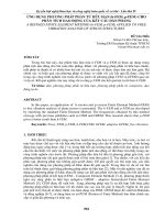
Fig. 4.1 illustrates the influence of grading indexes on the first four
natural frequency parameters of S-S beams with ∆T = 50K
20

5

µ2

µ1

4
3
2
2

1.5
n

1

x

0.5

0 0

0.5

1

1.5
n

15

10
2

2

1.5
n

z

40

1
x

0.5

0 0

0.5

1

1.5

2

n

z

60

µ4

µ3

50
30

40
20
2

1.5
nx

1

0.5

0 0

0.5

1.5

1

2

30
2

nz

1.5

1
n

x

0.5

0 0

0.5

1.5

1

2

n

z

Fig. 4.1. Influence of grading indexes on the first four natural frequency parameters of
S-S beams with ∆T = 50K

From Fig. 4.1 ones can see that:
- At a given value of the index nx , the fundamental frequency parameter µ1 tends to decreased by the increase in the index nz . The decrease

of µ1 is more significant for the beam with a higher index nx . The effect
of the index nx on the fundamental frequency parameter is different from
that of the index nz , and µ1 increases with the increase of the nx index.
However, the increase of µ1 is more significant for the beam associated
with a lower index nz .
- The fundamental frequency parameter attains a maximum value at
nx = 2 and nz = 0, and this is the special case when the beam degrades to
the axially FG beam made of the two ceramics.
- At the given value of the temperature rise, the effect of the grading
indexes on the higher frequency parameters is similar to the case of the
fundamental frequency parameter, they are also decreased by increasing
the index nz and they are increased by increasing index nx .
4.2.1.2. Influence of temperature rise
Fig. 4.2 illustrates the influence of grading indexes on the fundamental
frequency parameters of S-S beams for various temperature rise ∆T .
Some comments can be drawn from Fig. 4.2 as follows:


16

5

4

4

µ

1

µ1

5

3

3
2
2

1.5
nx

1

0.5

0 0

0.5

1

1.5

2
2

2

1.5
nx

nz

1

0.5

(a) ∆T=0 K

0.5

1.5

2

n

z

(a) ∆T=20 K

5

5

4
µ1

µ1

4

3
2
2

0 0

1

3
1.5
n

x

1

0.5

0 0

0.5

1

1.5
nz

2

2
2

1.5

1

n

0.5

x

(c) ∆T=40 K

0 0

0.5

1

1.5

2

n

z

(d) ∆T=80 K

Fig. 4.2. Influence of grading indexes on µ1 of S-S beams for various temperature rise
∆T

- The relation between the grading indexes and frequency parameters
unchanged when the value of ∆T increases. That means, the frequency
parameters decrease when increasing the index nz and they increased with
increasing the index nx . However, this relation is affected by the temperature rise. In particular, when nz increases from 0 to 2, the fundamental frequency parameters of the beam is significantly decrease, especially
when the index nx is large.
- The fundamental frequency parameters of beams is significantly decrease when the value of the ∆T increases.
4.2.1.3. Influence of the boundary conditions
Some comments can be drawn from this section as follows:
- The frequency parameters of the C-C beam is highest while that one
of C-F beams is lowest. At the reference temperature (∆T = 0K), the
variation of the frequency parameters with the grading indexes of the C-C
beam and the C-F beam is similar to that of the S-S beam. However, the
C-F beam is more sensitive to the change in the index nx than the S-S and
C-C beams, especially when nz is small.


17

- The effect of the grading indexes on the higher frequency parameters
of the C-C beam and the C-F beam is similar to that of the S-S beam.
- The variation of the frequency parameters of C-C and C-F beams
with values of the temperature rise are similar to S-S beams. However,
this variation is strongly influenced by boundary conditions. Specifically,

C-C beams are less affected by temperature rise. In contrast, C-F beams
are very sensitive to the rise of temperature.
4.2.1.4. Influence of the aspect ratio

1

4.5
4
3.5
3
2.5
2
1.5
2

µ

µ1

The effect of the beam aspect ratio, L/h, on the fundamental frequency
parameters of the beam is illustrated in Fig. 4.7, where the variations of
the fundamental frequency parameter with the grading indexes of the SS beam are depicted for two values of the aspect ratio, L/h = 10 and
L/h = 30, and for a temperature rise ∆T = 50K.
In Fig. 4.7, the relation between the grading indexes and frequency parameters unchanged when the value of L/h increases, means an increase
in the aspect ratio leads to a significantly decrease of the fundamental frequency parameter. It should be noted that previous studies have shown
that when beams are placed at reference temperature, an increase in the
aspect ratio leads to a significantly increase of the fundamental frequency
parameter. However, as shown in Fig. 4.7, this is no longer true when the
effect of temperature is considered. This can be explained by the fact that
when beams are placed in temperature environments, the stiffness of the

beams with high aspect ratio is significantly decrease than that of beams
with low aspect ratio .

1.5
nx

1
0.5

0.5
0 0
(a) ∆T=50 K, L/h=10

1

1.5
n

z

2

4.5
4
3.5
3
2.5
2
1.5
2

1.5
n

1
x

0.5
0 0

0.5

1

1.5

2

nz

(b) ∆T=50 K, L/h=30

Fig. 4.7. Variation of fundamental frequency parameter with grading indexes of S-S
beam in thermal environment with different values of aspect ratio


18

4.2.1.5. Mode shapes
Fig. 4.8 illustrates the first three mode shapes for u0 , w0 and γ0 of SS beams with two pairs of the grading indexes: (nx , nz ) = (0.0, 0.5) and
(nx , nz ) = (0.5, 0.5), in the reference temperature (∆T = 0).

1.5

w

mode 1

1.5
mode 1

0

u

1

0

γ0

0.5
0

1
0.5
0

n =0, n =0.5
x

−0.5

n =0.5, n =0.5

z

0

0.25

0.5

0.75

−0.5

1

mode 2

1

0.5

0.75

1

0.25

0.5

0.75

1

0.25

0.5

0.75

0.5

0

0

−0.5

−0.5
−1

−1
−1.5

0
1.5

0.25

0.5

0.75

−1.5

1

0

1.5

mode 3

1

1

0.5

0.5

0

0

−0.5

−0.5

−1
−1.5

z

0.25
mode 2

1

0.5

(a)

x

0

1.5

1.5

mode 3

−1
0

0.25

0.5

0.75

1

−1.5
(b)

0

1

Fig. 4.8. The first three mode shapes for u0 , w0 and γ0 of S-S beams with ∆T = 0K: (a)
(nx , nz ) = (0, 0.5), (b) (nx , nz ) = (0.5, 0.5)

As can be seen from the figure, the mode shapes of the 2-D FGM beam
as depicted in Fig. 4.8(b) are very different from that of the unidirectional
transverse FGM beam as depicted in Fig. 4.8(a). While the first and third
modes of the transverse displacement w0 of 1D-FGM beam are symmetric
with respect to the mid-span, that of the 2D FGM beam are not. The figure
also shows the difference in the mode shape of u0 and γ0 of the 2-D FGM
beam with that of the 1D beam, and the asymmetric of the second mode
for γ0 with respect to the mid-span is clearly seen from Fig. 4.8(b). Thus,
the variation of the constituent materials in the longitudinal directions
has a significant influence on the vibration modes of the beam. The mode
shapes for u0 , w0 and γ0 of the S-S 2D-FGM beam in thermal environment
are also considered for various values of the grading indexes. The grading
indexes and temperature rise have a significant influence on the vibration
modes of the beam, and not only vibration amplitude but also the position
of the critical point is changed.

4.2.2. Tapered beams


19

4.2.2.1. Influence of material distribution
The influence of the grading indexes on the frequency parameter received for tapered 2D-FGN beams is similar to constant cross-section
beams. However, the longitudinal index nz have less effect on the fundamental frequency parameter of tapered beams compared to constant
cross-section beams, especially with C-F boundary beam tapered beams.
4.2.2.2. Influence of taper ratio and taper case
The taper ratio versus the fundamental frequency parameter of the tapered 2D-FGM beam with nz = 0.5 and different values of nx is depicted
in Figs. 4.14-4.16 for the C-F, S-S and C-C beams, respectively. As can
be seen from the figures, the variation of the frequency parameter with
the taper ratio is governed by the boundary conditions and the taper case
as well. While the frequency parameter of the C-F beam increases by
increasing the taper ratio, that of the S-S and C-C beams decreases with
the increase of the taper ratio, regardless of the taper case. For a given
boundary condition, the dependence of the frequency parameter upon the
taper ratio c is, however significantly influenced by the taper case. The
rate of the variation of µ1 with is the most significant for the type C of
the C-F and S-S beams, while that is occurred for the type B of the C-C
beam.
4.2.2.3. Influence of aspect ratio
Some comments can be drawn from this section as follows:
- The effect of the aspect ratio on the frequency of the tapered beam is
less significant than that of the uniform beam.
- The effect of the aspect ratio on the frequency is also influenced by
the boundary condition, and the increase of the fundamental frequency of
the S-S beam is more significant than that of the C-F beam, regardless of
the grading indexes and the taper ratio.

4.3. Forced vibration
4.3.1. Influence of the moving load speed
In Fig. 4.17, the time histories for normalized mid-span deflection,
w0 (L/2,t)/wst , of the 2D-FGM beam are depicted for various values of
the moving load speed v and the indexes nx and nz . In the Figure, the midspan deflection is normalized by the static deflection of the isotropic beam


20

3

3
Case A
Case B
Case C

2

µ

µ

2
1.5

1.5
(a) n =0, n =0.5

1

x

0

0.3

z

0.6

1

0.9

c

3

0.3

1

0.6

0.9

0.6

0.9

c
Case A
Case B
Case C

2.5

2

µ

2

1.5

1.5
(c) n =2, n =0.5

1

(b) nx=0.5, nz=0
0

3

Case A
Case B
Case C

2.5

µ1

Case A
Case B
Case C

2.5
1

1

2.5

x

0

0.3

0.6

(d) n =0.5, n =2

z

1

0.9

x

z

0

0.3

c

c

Fig. 4.14. Taper ratio versus fundamental frequency parameter of C-F beam with
different taper cases and grading indexes:: (a) (nx , nz ) = (0, 0.5), (b) (nx , nz ) = (0.5, 0),
(c) (nx , nz ) = (2, 0.5), (d) (nx , nz ) = (0.5, 2)
5

5

(a) n =0, n =0.5
x

(b) n =0.5, n =0

z

x

1

3

Case A
Case B
Case C

2

1

z

4

µ

µ

1

4

0

3
Case A
Case B
Case C

2

0.3

0.6

1

0.9

0

0.3

5
x

x

0.9

z

4
1

3

µ

1

0.6

(d) n =0.5, n =2

z

4

µ

0.9

5
(c) n =2, n =0.5

Case A
Case B
Case C

2
1

0.6
c

c

0

3
Case A

Case B
Case C

2

0.3

0.6
c

0.9

1

0

0.3
c

Fig. 4.15. Taper ratio versus fundamental frequency parameter of S-S beam with
different taper cases and grading indexes:: (a) (nx , nz ) = (0, 0.5), (b) (nx , nz ) = (0.5, 0),
(c) (nx , nz ) = (2, 0.5), (d) (nx , nz ) = (0.5, 2)

made of aluminum. The moving load speed, as seen from the Figure,
affects both the dynamic deflection and the way the beam vibrates. For


21

7

7
µ

1

9

µ1

9

(a) n =0, n =0.5
x

5

3

(b) n =0.5, n =0
x

z

5

Case A
Case B
Case C
0

0.3

0.6

3

0.9

z

Case A
Case B
Case C
0

0.3

c

0.6

0.9

0.6

0.9

c

9

9

µ

µ

1

7

1

7
(c) n =2, n =0.5
x

5

3

0

(d) n =0.5, n =2

z

x

5

Case A
Case B
Case C
0.3

0.6

0.9

3

z

Case A
Case B
Case C
0

c

0.3
c

Fig. 4.16. Taper ratio versus fundamental frequency parameter of C-C beam with
different taper cases and grading indexes:: (a) (nx , nz ) = (0, 0.5), (b) (nx , nz ) = (0.5, 0),
(c) (nx , nz ) = (2, 0.5), (d) (nx , nz ) = (0.5, 2)

the given values of the grading indexes, the beam shows more vibration

cycles when it is subjected to the lower moving speed load. The grading
indexes considerably affect the dynamic deflection of the beam, but they
hardly affect curve shapes of the time histories.
4.3.2. Influence of material distribution
In Fig. 4.18, the relation between the dynamic magnification factor
and the moving load speed is illustrated for various values of the indexes
nz and nx . As seen from the Figure, the relation between Dd and v of
the 2D-FGM beam is similar to that of an isotropic beam under a moving load, that is, the factor Dd both increases and decreases, and it then
monotonously increases to a maximum value when increasing the moving load speed. The repeated increase and decrease of the factor Dd for
lower values of the moving load speed in Fig. 4.18, as mentioned above,
is associated with the oscillations of the beam under the load with the
lower moving load speed to the critical speed ratios. The effect of the
grading index nz on the factor Dd is, however, different from that of the
index nx . The dynamic magnification factor steadily decreases as the index nx increases, whereas it increases by the increase in the index nz . The
effect of the two grading indexes on the factor Dd can be explained by


0.6

0.6

0.4

0.4
w0(L/2,t)/wst

w0(L/2,t)/wst

22

0.2
v=20 m/s
v=50 m/s
v=100 m/s

0
−0.1

0.2

0

0.2

0.4

0.6

v=20 m/s
v=50 m/s
v=100 m/s

0
0.8

1

(a)

−0.1

(b)

0

0.2

t/∆T*

st

0.4

0.1

v=20 m/s
v=50 m/s
v=100 m/s

0
−0.2

0.2

w (L/2,t)/w

w0(L/2,t)/wst

0.8

(c)

0.8

1

0.8

1

0.3

0

1.2

0.4
0.6
t/∆T*

0

0.2

0.4
t/∆T*

0.6

v=20 m/s
v=50 m/s

v=100 m/s

0
0.8

1

−0.05
(d)

0

0.2

0.4
0.6
t/∆T*

Fig. 4.17. Time histories for normalized mid-span deflection with different indexes nx
and nz : (a) (nx , nz ) = (1/3, 1/3), (b) (nx , nz ) = (3, 3), (c) (nx , nz ) = (0, 3), (d)
(nx , nz ) = (3, 0)

the dependence of the rigidities on these indexes. The beam associated
with a higher index nx contains more C1 and M1, and thus, its rigidities
are higher, whereas the rigidities of the beam with a higher index nz are
lower.
The thickness distribution of the normalized axial stress at mid-span
section of the 2D-FGM beam is depicted for v = 100 m/s and various values of the grading indexes. The stress in the Fig. 4.20 was computed at
the time when the load arrives at the mid-span, and it was normalized as
σ ∗ = σxx /σ0 , where σ0 = PLh/8I. The thickness distribution of the stress

of 2D-FGM beam, as seen from the Figure, is very different from that of
isotropic beams, and the stress does not vanish at the mid-span, except for
the case nz = 0, which corresponds to the axially FG beam composed of
the two ceramics. The influence of the index nz on the stress distribution
is also very different from that of the index nx . The maximum amplitude of both the compressive and tensile stresses decreases as the index
nx increases, whereas it increases as the index nz increases. Thus, by raising the index nx , we could decrease not only the dynamic magnification


23

0.9

0.9

nx=0
nx=1/3
nx=1
nx=3

nz=1/3
0.8
0.7

nx=1/3
0.8
0.7

0.6
D

d

Dd

0.6

0.5

0.5

0.4

0.4

0.3

0.3
(a)

0.2

0

50

100

150

200

250

300

nz=0
nz=1/3
nz=1
nz=3

(b)

350

0.2

0

50

100

150

200

250

300

350

v (m/s)

v (m/s)

Fig. 4.18. Relation between dynamic magnification factor and moving load speed with
different indexes: (a) nz = 1/3, nx is variable; (b) nx = 1/3, nz is variable
0.5

0.5
n =0

n =0

n =1/3

n =1/3

x

z

x

z

nx=1

0.25

nz=1

0.25

nz=3
z/h

z/h

nx=3
0

−0.25

0

−0.25

(b) n =1/3

(a) n =1/3
−0.5
−2

z

−1

0

σ*

1

2

−0.5
−2

x

−1

0
σ*

1

2

Fig. 4.20. Thickness distribution of normalized axial stress at mid-span section for
v = 100 m/s: (a) nz = 1/3, nx is variable, (b) nx = 1/3, nz is variable

factor, but also the maximum amplitude of the axial stress.
Conclusion of Chapter 4
On the basis of comparing the numerical results obtained in the thesis
and the published results, Chapter 4 has proved that all four FE models
developed in the thesis are reliable in evaluating the vibration characteristics of FGM beams. Three FE models are confirmed to have high
convergence rate, namely FBKo, FBHi and TBSγ models, while TBSγ
model has a much slower convergence rate. Using the FE models and

the numerical calculation program, Chapter 4 analyzed free vibration and