SPATIAL DISTRIBUTION OF OVERTOPPING
Bạn đang xem bản rút gọn của tài liệu. Xem và tải ngay bản đầy đủ của tài liệu tại đây (939.39 KB, 13 trang )
SPATIAL DISTRIBUTION OF OVERTOPPING
Anestis Lioutas1, Gregory M. Smith1, Henk Jan Verhagen2
The scope of this research is to find an empirical formula to describe the distribution of wave overtopping in the
region behind the crest. A physical model was set up in which irregular waves were generated. In order to find a
formula which adequately describes the test observations, the influence of several parameters has been analysed. The
proper determination of the crest freeboard, which is a dominant factor, has been investigated. Finally, the test results
have been used to assess and compare the existing relevant computational methods.
Keywords: overtopping; rubble-mound breakwater; physical modelling; spatial distribution; crest freeboard
INTRODUCTION
The initial goal of this study was to develop a computational tool to calculate the wave overtopping
discharge at certain point behind the crest of a simple rubble mound breakwater without any crest
element (Figure 1). The computational methods of wave overtopping which are included in the coastal
guidelines and manuals have been developed to calculate the discharge at top of the crest. However, for
the design of some coastal protection structures the maximum tolerable discharge is specified at a
certain point behind the crest. Therefore, the spatial distribution of overtopping can become an issue
with significant impact on the design of the structure.
Figure 1. Research objectives.
This topic has been studied by Juul Jensen (1984), Besley (1999) and Lykke Andersen (2006) for
different structural configurations. Juul Jensen’s research was based on physical model tests of several
rubble mound breakwater types. Lykke Andersen (2006), also based on a large physical modelling
dataset, investigated the landward distribution of breakwaters with a crest element. Besley (1999)
described the influence of a wide crest on the overtopping discharge by introducing a reduction factor.
The last two methods are included in the EurOtop Manual (2007).
All the existing computational methods for overtopping are purely empirical. Thus, a similar
approach to the previous studies has been used in this research, by means of experimental 2D testing. A
physical model of a typical rock breakwater or revetment was set up in the wave flume of the Fluid
Mechanics Laboratory of the TU Delft.
PHYSICAL MODEL
Wave flume
The experiments have been performed in the at the wave flume “Lange Speurwerk Goot” at the
Fluid Mechanics Laboratory of the TU Delft. It has a length of 40m and a cross-section of 0.80m x
0.80m (width x height). The wave generator in this flume operates with mechanical pressure. It is a
second order wave generator which means that the second-order effects of the first higher and first
lower harmonics of the wave field are taken into account in the wave generator motion. It is also
1
2
Van Oord n.v.– Dredging and Marine Contractors, Schaardijk 211, Rotterdam, Netherlands
Hydraulic Engineering Department, TU Delft, Stevinweg 1, Delft, Netherlands
1
2
COASTAL ENGINEERING 2012
equipped with Active Reflection Compensator (ACR) which reduces the wave reflection. The wave
generator is controlled with the use of DASYLab, software developed by National Instruments®. The
function of the generator is determined by a steering file which contains all the wave information: the
requested wave height and period, the type of the spectrum (JONSWAP, Pierson/Moscowitz, simple
sinusoidal etc.), its characteristics (peak-enhancement factor, peak-width factor) and the duration. In
this research only JONSWAP spectra have been generated changing only the peak-enhancement factor
from 3.3 to 9 for wind and swell waves accordingly.
Prototype and scale model
The prototype structure was a conventional rubble mound breakwater with a double rock layer on a
permeable core. Since the scope of this study was the basic understanding of the overtopping processes,
no further configurations (crest elements, toe or berm) have been considered. The hydraulic stability of
the structure was determined with the use of the method proposed in the Rock Manual.
To fit properly in the wave flume the prototype structure was scaled with a factor 1:20. The rock
properties were Dn50=60mm and 25mm for armour layer and core respectively. The slope of the
structure varied from 1:1.5 to 1:3. The armour layer thickness and the crest width were determined
according to the Rock Manual; ie. 2*Dn50 and 3*Dn50, respectively. The crest level of the model was
held constant and the freeboard was varied by adjusting the water level. The dimensions of the model
are presented in the next figure (Figure 2).
Figure 2. Physical model properties
Figure 3. Pictures of the scale model
Measuring system
A number of important issues had to be tackled in this model set-up. The first was that the
measurement of the water in several locations behind the crest should be done within the same
experiment in order to keep the test conditions constant for each experiment. To measure the
overtopping discharge at several points simultaneously a series of splitting bins were installed in the
backfill (the area behind the crest), separating the area into 6 sectors (see Figure 4). Since from the
COASTAL ENGINEERING 2012
3
related literature it was known that the decay of the overtopping is exponential, the width of these bins
was not constant. The first two bins were 0.05m wide, the next two 0.10m and the last two 0.20m.
The next and more important issue which had to be solved was the water loss during the
experiment. To measure the overtopping water it is extracted from the flume leading to (significant in
this case) water loss. This loss results in reduction of the water level in the flume which means that the
crest freeboard, which is one of the most influential factors, would not remain constant during the
experiment.
This problem has been solved by storing the collected overtopping water into floating tanks behind
the structure (collecting tanks – see Figure 4). In that way, the water which is initially collected into the
splitting bins (sectors) is pumped into the floating tanks (one for each bin/sector). The free water flow
through the core and below the bins ensured the equalisation of the water level in front and behind the
model. In fact, the overtopping water stays inside the flume; it is only separated from the rest of the
water. In this way the total amount of water in the flume was maintained during the experiment and the
water level at the sea side of the model did not reduce because of the collection of overtopping water.
Thus, the crest freeboard remained constant during the whole procedure.
Figure 4. Measuring system
Test set-up and programme
Four parameters were varied in this research: the wave height, the wave steepness (period), the
crest freeboard and the slope of the structure. The tested range of each parameter is listed below.
Wave height: 0.08-010m (swells), 0.12m, 0.14m, 0.16m and 0.18m.
Wave steepness: 1/20 (=0.05), 1/35 (≈0.03), 1/50 (=0.02) and 1/200 (=0.005 – swells).
Crest freeboard: 1·Hs and 1.5·Hs. For the swells: 2·Hs.
Slope tanα: 1:1.5, 1:2 and 1:3
Each test consisted of a wave train of 1000 waves approximately. The generated spectrum was
JONSWAP with peak enhancement factor equal to γ = 3.3 for all the experiments except from those
with swell. In that case γ = 9.
During the literature study some ambiguities were found in the definition of the crest freeboard
between different guidelines. To investigate this issue the entire test programme was later repeated (by
Z. Afridi) with a “closed” (impermeable) crest as shown in the next figure.
4
COASTAL ENGINEERING 2012
Figure 5. “Closed” – impermeable crest.
REASULTS ANALYSIS
According to the existing relevant literature, the main input for the computation of the spatial
distribution is the total overtopping. Although this process has been thoroughly studied by many
researchers it is important to investigate the most suitable way to introduce it in this study and to use it
in order to develop a computational formula for the spatial distribution. For this reason, even though the
main topic of this research is the overtopping behind the crest, a large part of the analysis has been
dedicated to the total overtopping.
Crest freeboard definition
According to the relevant literature two different definitions of the crest freeboard exist. The
standard definition is described in the most of the guidelines as the vertical distance between the top
horizontal part of the crest and the still water level. In Figure 6 it is defined as Ac. It must be noted that
since the armour has a relatively rough surface, the determination of “the top horizontal part of the
crest” can vary depending on the measuring method and equipment (e.g. semi-spherical or point staff).
To avoid any confusion on this issue, in this research this level has been determined as the level of a
thin plate placed on top of the crest and it coincides basically with the top part of the stones. This is
commonly used as the “design crest level”. The other methods result in slightly lower levels.
In the EurOtop Manual it is suggested that for rubble mound structures without a crest element, the
upper limit is the top level of the (impermeable) backfill or underlayer and not the top level of the
rubble mound armouring. (The latter distance is called armour freeboard Ac). Thus the crest freeboard
in this case is defined as the distance from still water level to the upper non (or only slightly) waterpermeable layer (Rc in Figure 6).
Figure 6: Crest freeboard definition according to EurOtop Manual
According to these definitions for the original scale model (see Figure 2) the freeboard is:
0,15m (standard definition, the permeable crest is taken into account)
0,03m (EurOtop suggestion, the permeable crest is not considered).
COASTAL ENGINEERING 2012
5
Figure 7 presents the data collected for the 1:2 slope using both definitions. In this graph, the data
from tests with impermeable crest are also shown. (In this case there is no doubt about the freeboard:
the full crest level should be applied). The line shown in the figure is the theoretical overtopping
prediction using the EurOtop formula. All the data are plotted using the dimensionless parameters
proposed by EurOtop: Q*, dimensionless overtopping discharge and Rc*, dimensionless freeboard.
Figure 7: Total overtopping (in 1:2 slope) - Impact of the crest freeboard definition
The impact of the freeboard definition in this plot is apparent: depending the definition the
observations are shifted parallel to X-axis (Rc*).
When the EurOtop definition is applied a considerable difference has been observed between the
experimental data and the theoretical prediction. The prediction formula leads to significant
overestimation which can be explained by the fact that the entire crest has not been taken into account.
The use of the standard definition presented a better correlation with the theoretical line but a
general underestimation trend of the prediction formula has been observed. However this is expected
since the top layer of the crest is more permeable and allows more overtopping water to flow through it.
A better fit of the data with the theoretical line is achieved when the standard-defined freeboard has
been used reduced by 0.9∙Dn50 (denoted as Ac' = Ac – 0.9∙Dn50 in Figure 7). Note that this reduction
applies when the top level is measured in the previously described way.
In Figure 6 the results of the test with the “closed” or impermeable crest have also been plotted.
They follow the same trend as the data with Ac' and they present an equally good fit with the EurOtop
formula. This correlation enhances the idea that standard definition (Ac') better describes the conditions
of this model. For this reason the analysis of the test results has been performed using the adjusted
standard definition (Ac'). Since freeboard is always denoted as “Rc” in the entire relevant literature, to
avoid confusion, this notation will be kept in this research also (instead of Ac').
Total overtopping
For the computation of the total overtopping the EurOtop method has been used. This method
makes a distinction between breaking and non-breaking wave conditions. The parameters that
determine the whole process according to the method are:
wave height
wave period /steepness
crest freeboard
slope angle
roughness
angle of incident wave
The main difference between the two formulas is the that the breaking-wave formula takes into
account the wave steepness and the slope of the structure (with the introduction of the breaker number
ξm-1,0 – computed with Tm-1,0 ) contrary to the non-breaking-wave formula, which implies that these two
factors do not have any influence on the total overtopping.
6
COASTAL ENGINEERING 2012
The wave conditions applied in the entire experimental process have been chosen to be nonbreaking (the breaker number ξm-1,0 > 2 in all the tests) and thus according to the relevant formula of
EurOtop the wave steepness and the slope of the structure shall not be taken into account. To obtain a
better insight into the prediction method the influence of these parameters is shown separately.
Impact of the wave steepness
Figure 8: Total overtopping (in 1:2 slope) - Impact of the wave steepness
The test results for the total overtopping on 1:2 slope are presented in Figure 8. In order to check
influence of the wave steepness (and period) on the prediction formula the observations are plotted
against the dimensionless parameters proposed by EurOtop.
The main observation on this graph is that the measured overtopping discharges are clearly grouped
according to wave steepness: longer waves produce larger overtopping and vice versa. Furthermore
these groups follow the same trend. This implies that the wave period has some influence on the total
overtopping.
Impact of the slope
Figure 9 presents the total overtopping measured for three different slopes: 1:1.5, 1:2 and 1:3. In
the graph, the EurOtop formula is also denoted.
From this graph, it can be observed the data are grouped according to slope. Generally, a vertical
shift of the data (parallel to y-axis) can be observed implying a relation between total overtopping and
slope: steeper slopes result in higher overtopping rates.
Figure 9: Total overtopping (all slopes) - Impact of the wave steepness
7
COASTAL ENGINEERING 2012
Compared to the EurOtop method, it seems that the prediction formula has a tendency to
overestimate the overtopping discharge for mild slopes (1:3 and milder) and to underestimate it for
steeper slopes (1:1.5).
EurOtop method - adjustment
The investigation of the impact of the wave steepness and slope showed that these two parameters
were not irrelevant with the total overtopping. The existence of a scatter (caused by the wave steepness
and slope) in the graphs presented above means that the dimensionless parameters (Q* and Rc*) do not
properly describe this influence of the wave period.
Since these two parameters are already introduced in the EurOtop formula for breaking waves (with
the use of the breaker number ξ), the first and more logical attempt to solve this issue is to use this
formula instead of the non-breaking which is suggested in the manual. The graph in Figure 8 present the
entire dataset plotted according to the breaking-wave formula. Note that the axes are adjusted
accordingly.
Figure 10: Total overtopping – Breaking-wave formula
This graph shows a better correlation between the measurements and the prediction, compared with
the graph plotted with the non-breaking-wave formula (Figure 8). The scatter is smaller and the
measurements lay closer to the EurOtop line. Even the data from tests with very long waves (swells)
stay closer to the other experiments and to the theoretical prediction line. This implies that wave
period/steepness is well introduced with the parameter Rc*/ξ0 (Rc*/ξm-1,0 ).
The second observation when comparing the these two graphs (Figure 8 and 10) is that while in
Figure 8 the non-breaking-wave formula was underestimating the results (especially for longer waves),
in the later it happens exactly the opposite: breaking-wave formula overestimates all the data, notably
those with small steepness (large period). This means that in the first case the breaker number is “underrepresented” and in the second “over-represented”.
The latest remark leads to the conclusion that an intermediate solution would solve this issue. Since
the only change between the two formulas is the breaker number ξ0, it is suggested to be raised in a
power k (with 0 < k <1). The constant values of the formulas are also linearly interpolated based on the
value of power k. The resulting formula is the following:
Q
gH
3
m0
k
R
1
(0.2 0.133 k ) b 0 exp (2.6 2.15 k ) c
k
H m 0 f ( b v 0 )
tan a
(1)
This formula is in fact a generic form of the standard EurOtop method which combines both
formulas: if power k is 1 the breaking-wave formula is formed and when k=0 the non-breaking-wave.
For the test results of this experimental research the k-value which presented the best fit was
k=0.60. According to EurOtop for this case the roughness factor γf should be 0.4 (for two layers of
armour stone over permeable core). A better fit has been achieved with γ f =0.45 which is reasonable
since the permeability of the core in this model has been affected from the wall of the splitting bin
8
COASTAL ENGINEERING 2012
installed under the crest (see Figure 4). The reduction factors for berm and vertical walls are 1 in this
case and thus it cannot be concluded from this study if they should be raised to the power k. For
mathematical consistency reasons they are presented in this form; however further investigation is
strongly recommended in case of structures with berm or vertical wall.
Figure 11 presents all the results plotted against the adjusted EurOtop formula (1). Note that both
axes have changed accordingly: the x-axis is Rc*/ξk (instead of Rc* or Rc*/ξ0) and the y-axis has
changed to Q*/(γb∙ξ0/√tanα)k. For practical reason the later will be denoted as Q*/ξ* in the graphs.
Figure 11: Total overtopping – Adjusted EurOtop formula (with k=0.6)
The graph in Figure 11 shows an improved fit of the results. No obvious grouping can be observed:
all the results (both for “open”/permeable and “closed” crest) follow the same trend which coincides
with the adjusted theoretical line. This leads to the conclusion that the breaker number (and thus the
wave steepness and slope) is properly introduced in the prediction formula.
Since with the adjusted formula a better correlation is achieved which means that the process is
better described, for the next steps of this research (determination of the spatial distribution) the total
overtopping will be computed using this method.
Spatial distribution
The landward region of coastal protection structures consists of two areas: the crest and the
backfill. These two surfaces have different physical characteristics (geometry, roughness and
permeability) and as consequense the flow of overtopping water on/through them may deviate. For this
reason, in order to define the spatial distribution in the backfill it is suggested to esstimate first the
overtopping directly behind the crest and use it as an input for the landward distribution.
Overtopping directly behind the crest
Initially the test results directly behind the crest are plotted with the adjusted EurOtop formula
(Figure 12a) in order to compare them with the total overtopping and have a first idea of the reduction.
The main obseravtion on this graph is first that the reduction in the water quantities is uniform and
secondly that the results follow a common trend which is similar to the total overtopping prediction.
The later leads to the conclusion that the same parameters are dominant in this case also and that the
prediction formula could be used as a basis to describe the overtopping at this point.
Similarly to the other reduction factors of the method (for berm, oblique waves, roughness and
vertical walls) a new reduction factor γc is proposed to be introduced in the adjusted EurOtop formula
(1):
k
R
Q
1
(2)
(0.2 0.133 k ) b 0 exp (2.6 2.15 k ) c
k
3
H
(
)
tan a
gH m 0
m0
f
b
v
0
c
In Figure 12b the test results are plotted relatively to the formula (2). The best fit has been achieved
for a γc=0.6.
COASTAL ENGINEERING 2012
9
Figure 12: Overtopping directly behind the crest – Adjusted EurOtop formula for a) γc=1 and b) γc=0.6
Spatial distribution
Since a correlation between the adjusted EurOtop formula (2) and the test findings was found (with
the introduction of reduction factor γc), the data collected for certain distances behind the crest will be
presented again in the same way.
For each point a range of values of γc have been tested in order to achieve the best fit. For locations
further from the crest, the spread of the results is larger. This is expected because at this points the
measured water quantities were very small and thus the relative error was large.
Figure 13: Overtopping at certain points behind the crest
10
COASTAL ENGINEERING 2012
In general it can be concluded that the test results follow the same trend as the prediction line and
they present a good correlation with the adjusted EurOtop formula.
It must be noted that the analysed dataset contains a large range of wave and structural conditions:
the breaker number ξ varies between 2 to more than 9, the slope varies from 1:1.5 to 1:3, different
freeboards and crest configurations (“open”/ “closed”) have been tested. However it is validated only
for this type of structure; even though this is a typical and representative structure, for different
configurations the use of this prediction formula shall be further studied.
Since according to the literature (Juul Jensen (1984)) one of the dominant parameters in the spatial
distribution is the crest width B (also denoted as Gc in literature e.g. EurOtop – Figure 6), the change of
new reduction factor γc is suggested to be plotted as a function of it (Figure 14). In this way γc is
expressed in a dimensionless form which makes it easier to be applied.
Figure 14: Distribution of the new reduction factor γc
From Figure 13 it is observed that the various γc values can be connected linearly with the
following simplified formula:
c 0.142
x
0.577
B
(3)
Remark: The distance starts measuring from the point where the crest ends. This means that for
x=0, the reduction factor for the overtopping directly behind the crest is calculated.
COMPARISON WITH EXISTING METHODS
The findings of this research has been analysed and compared with the most relevant methods on
this issue which are that of Juul Jensen (1984) and Besley (1999).
Juul Jensen
Juul Jensen’s method uses two main input parameters to predict the spatial distribution: the
overtopping intensity directly behind the crest and a β factor which is a function of crest width B.
Concerning the first parameter, it is derived from the total overtopping (not computed in the same way
as the EurOtop method). According to the result analysis presented previously this may lead to a
(considerable) overestimation. Thus to do a proper assessment of the method it is proposed to use the
overtopping-directly-behind-the-crest instead.
Since the number of tests was significant only the results of two representative tests are presented:
one with relatively steep waves (s=1/20) on 1:2 slopes (Figure 15a) and another with longer waves
(s=1/35)on slope 1:1.5 (Figure 15b).
COASTAL ENGINEERING 2012
11
Figure 15: Distribution of overtopping (comparison with Juul Jansen method)
Most of the comparison graphs presented the same pattern as Figure 15a. Form these graphs it can
be seen that the Juul Jensen method (with the proposed adjustment) describes reasonably well the
distribution of overtopping. The shape of the decay coincides with both measured and predicted with
adjusted EurOtop formula. Some tendency for overestimation has been observed when compared with
the results of this research but generally the deviation was not considerable in most of the cases.
Figure 16 presents an overall comparison between the measured and the computed with Juul Jensen
method results.
Figure 16: Comparison between Juul Jensen and measured overtopping
The largest spread is observed for smaller overtopping discharges. In reality though this difference
is trivial (in the order to magnitude of 10-4 -10-5 l/s/m) and it can be explained by the fact that these test
results concerned very small water quantities where the accuracy in the measurement has been
dominated by model effects.
Besley
Besley’s method is included in the EurOtop Manual as a simple way to describe the effect of a wide
crest. The idea is to use a factor Cr to express the reduction of total overtopping at certain distance.
Figure 17 presents the test results with the use of the Besley method.
12
COASTAL ENGINEERING 2012
Figure 17: Overtopping distribution (Besley method)
This graph shows that no correlation between the predicted and measured data exists. The shape of
the decay (exponential) is well predicted but the spread of the result is significant. This can be
explained by the fact that this method takes into account only the wave height. Furthermore it was not
originally developed to predict the distribution of overtopping but the effect of a wide crest.
CONCLUSIONS AND RECOMMENDATIONS
The main goal of this research has been to study, by means of physical modelling, the spatial
distribution of overtopping in the area behind the crest. The main input of this process is the total
overtopping and thus it has been further investigated. From the study the following can be concluded:
The standard crest freeboard definition reduced by 0.9∙Dn50 presented better results compared with
the EurOtop definition.
The total overtopping has been better described with an adjusted version of EurOtop formula:
Q
gH m3 0
k
R
1
(0.2 0.133 k ) b 0 exp (2.6 2.15 k ) c
k
H m 0 f ( b v 0 )
tan a
(1)
For the test results of this study the best fit has been achieved for k=0.6.
For the spatial distribution a new reduction factor γc is introduced in the adjusted EurOtop formula:
Q
gH m3 0
k
R
1
(0.2 0.133 k ) b 0 exp (2.6 2.15 k ) c
k
H m0 f ( b v 0 ) c
tan a
(2)
This factor is expressed as a function of crest width B and can be determined by the following
formula:
x
(3)
0.142 0.577
c
B
The Juul Jensen (1984) method presents good correlation compared with the test results when the
overtopping-directly-behind-the-crest is used as an input instead of the total overtopping.
No correlation between the Besley (1999) method and the adjusted EurOtop could be found.
Based on the findings of this study the following recommendations are given:
The analysed dataset contains a large range of wave and structural conditions: the breaker number ξ
varies between 2 to more than 9, the slope varies from 1:1.5 to 1:3, different freeboards and crest
configurations (“open”/ “closed”) have been tested. However it is validated only for this type of
structure; even though this is a typical and representative structure, for different configurations the
use of this prediction formula shall be further studied.
COASTAL ENGINEERING 2012
13
The effect of other parameters such as berm, oblique waves, crest width etc. are not taken into
account; for such cases the presented theory shall be further studied.
ACKNOWLEDGMENTS
The contribution of Zirgham Afridi (exchange MSc student from Imperial College, UK at the time
that the physical modelling had been performed) who conducted part of the experimental procedure
(“closed”/impermeable crest tests) is greatly acknowledged. The comments and corrections made by
Jan Kees Krom, MSc student at TU Delft and intern in Van Oord, are highly appreciated.
REFERENCES
Besley, P. 1999. Overtopping of seawalls: design and assessment manual, R&D Technical Report No.
W178, Environmental Agency, Bristol.
Bruce, T., v.d. Meer, J.W., Franco, L., Pearson, J.M. 2009. Overtopping performance of different
armour units for rubble mound breakwaters, Coastal Engineering, vol.56, 166-179.
CIRIA, CUR, CETMEF. 2007. The Rock Manual. The use of rock in hydraulic engineering (2nd
edition), C683, CIRIA, London.
EurOtop. 2007. Wave overtopping of the sea defence and related structures: Assessment manual. EA
(UK), ENW (NL), KFKI (DE), ISBN 978-3-8042-1064-6
Hughes, S. 1993. Physical model and laboratory techniques in coastal engineering, World Scientific,
ISBN 981-02-1540-1
Juul Jensen, O. 1984. A monograph on rubble mound breakwaters, Danish Hydraulic Institute,
Horsholm.
Lioutas, A. 2010. Experimental research on spatial distribution of overtopping, MSc Thesis, Delft
University of Technology, Faculty of Civil Engineering and Geosciences, Delft.
Lykke Andersen, T., Burcharth, H.F. 2006. Hydraulic response on rubble mound breakwaters, Aalborg
University
Van Kester, D. 2009. Spatial distribution of wave overtopping, MSc Thesis, Delft University of
Technology, Faculty of Civil Engineering and Geosciences, Delft.