Introduction to fluid mechanics - P9

Drag and lift
In Chapters 7 and 8 our study concerned ‘internal flow’ enclosed by solid
walls. Now, how shall we consider such cases as the Aight of a baseball or
golf ball, the movement of an automobile or when an aircraft flies in the air,
or where a submarine moves under the water? Here, flows outside such solid
walls, i.e. ‘external flows’, are discussed.

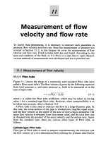
Generally speaking, flow around a body placed in a uniform flow develops a
thin layer along the body surface with largely changing velocity, Le. the
boundary layer, due to the viscosity of the fluid. Furthermore, the flow
separates behind the body, discharging a wake with eddies. Figure 9.1 shows
the flows around a cylinder and a flat plate. The flow from an upstream point
a is stopped at point b on the body surface with its velocity decreasing to
zero; b is called a stagnation point. The flow divides into the upper and lower
flows at point b. For a cylinder, the flow separates at point c producing a
wake with eddies.
Let the pressure upstream at a, which is not affected by the body, be pbo,
the flow velocity be U and the pressure at the stagnation point be p o . Then
P u2

Po=Poa+T

Fig. 9.1 Flow around a body

(9.1)


The drag of a body 149

Whenever a body is placed in a flow, the body is subject to a force from the
surrounding fluid. When a flat plate is placed in the flow direction, it is only

subject to a force in the downstream direction. A wing, however, is subject to
the force R inclined to the flow as shown in Fig. 9.2. In general, the force R
acting on a body is resolved into a component D in the flow direction U and
the component L in a direction normal to U. The former is called drag and
the latter lift.
Drag and lift develop in the following manner. In Fig. 9.3, let the pressure
of fluid acting on a given minute area dA on the body surface be p, and the
friction force per unit area be z. The force pdA due to the pressure p acts
normal to dA, while the force due to the friction stress z acts tangentially.
The drag D,, which is the integration over the whole body surface of the
component in the direction of the flow velocity U of this force p dA, is called
form drag or pressure drag. The drag D/ is the similar integration of zdA
and is called the friction drag. D, and D/ are shown as follows in the form of
equations:

D,=

J, pdAcos8

(9.2)

zdAsin8

(9.3)

4,

D -

The drag D on a body is the sum of the pressure drag D, and friction drag

Or, whose proportions vary with the shape of the body. Table 9.1 shows the

contributions of D, and D, for various shapes. By integrating the component
7
,
of pd.4 and ~ d . 4
normal to 1 the lift L is obtained.

Fig. 9.2 Drag and lift

Fig. 9.3 Force acting on body

9.3.1 Drag coefficient
The drag D of a body placed in the uniform flow U can be obtained from eqns
(9.2) and (9.3). This theoretical computation, however, is generally difficult
except for bodies of simple shape and for a limited range of velocity.


150 Drag and lift

Table 9.1 Contributions of &and Df for various shaoes

Therefore, there is no other way but to rely on experiments. In general, drag
D is expressed as follows:
PU‘
D = CDA2

(9.4)

where A is the projected area of the body on the plane vertical to the

direction of the uniform flow and C, is a non-dimensional number called
the drag coefficient. Values of C, for bodies of various shape are given in
Table 9.2.

9.3.2 Drag for a cylinder
Ideal fluid
Let us theoretically study (neglecting the viscosity of fluid) a cylinder placed
in a flow. The flow around a cylinder placed at right angles to the flow U of
an ideal fluid is as shown in Fig. 9.4. The velocity uo at a given point on the
cylinder surface is as follows (see Section 12.5.2):
v8 = 2U sin0

(9.5)

Putting the pressure of the parallel flow as pm, and the pressure at a given
point on the cylinder surface as p, Bernoulli’s equation produces the
following result:

u2
Pd
+P2 +2

pm -= p
P-Pm=
-’-Po,

PU2/2

p(U2 - Ui) --2 (1 -4sin28)
- pu’

2
- 1 -4sinz0

(9.6)


The drag of a body 151

Table 9.2 Drag coefficients for various bodies


152 Orag and lift

Fig. 9.4 Flow around a cylinder

Fig. 9.5 Pressure distribution around cylinder: A, Re = 1.I x 10’ < Re,; B, Re = 6.7 x 1O5 > Re,;
C, Re = 8.4 x lo6 > Re,

This pressure distribution is illustrated in Fig. 9.5, where there is left and
right symmetry to the centre line at right angles to the flow. Consequently the
pressure resistance obtained by integrating this pressure distribution turns
out to be zero, i.e. no force at all acts on the cylinder. Since this phenomenon
is contrary to actual flow, it is called d’alembert’s paradox, after the French
physicist (1717-83).


The drag of a body

Wscous fluid
For a viscous flow, behind the cylinder, for very low values of Re < 1

(Re = Ud/u), the streamlines come together symmetrically as at the front
of the cylinder, as indicated in Fig. 9.4. If Re is increased to the range
2 30 the boundary layer separates symmetrically at position a (Fig. 9.6(a))
and two eddies are formed rotating in opposite directions.' Behind the eddies,
the main streamlines come together. With an increase of Re, the eddies
elongate and at Re = 40 70 a periodic oscillation of the wake is observed.
These eddies are called twin vortices. When Re is over 90, eddies are
continuously shed alternately from the two sides of the cylinder (Fig. 9.6(b)).
Where lo2 < Re < lo5, separation occurs near 80" from the front stagnation
point (Fig. 9.6(c)). This arrangement of vortices is called a Karman vortex
street. Near Re = 3.8 x lo5, the boundary layer becomes turbulent and the
separation position is moved further downstream to near 130"(Fig. 9.6(d)).
For a viscous fluid, as shown in Fig. 9.6, the flow lines along the cylinder
surface separate from the cylinder to develop eddies behind it. This is
visualised in Fig. 9.7. For the rear half of the cylinder, just like the case of a
divergent pipe, the flow gradually decelerates with the velocity gradient
reaching zero. This point is now the separation point, downstream of which
flow reversals occur, developing eddies (see Section 7.4.2). This separation
point shifts downstream as shown in Fig. 9.6(d) with increased Re = U d / u (d:
cylinder diameter). The reason is that increased Re results in a turbulent
boundary layer. Therefore, the fluid particles in and around the boundary
layer mix with each other by the mixing action of the turbulent flow to make

-

-

Fig. 9.6 Flow around a cylinder

'

Streeter, V.L., Handbook o Fluid Dynamics, (1961), McGraw-Hill, New York.
f

153


154 Drag and lift

Fig. 9.7 Separation and Karman vortex sheet (hydrogen bubble method) in water, velocity 2.4cm/s,
Re= 195

separation harder to occur. Figure 9.8 shows a flow visualisation of the
development process from twin vortices to a Kkrman vortex street. The
Reynolds number Re = 3.8 x lo5 at which the boundary layer becomes
turbulent is called the critical Reynolds number Re,.
The pressure distribution on the cylinder surface in this case is like curves
A, B and C in Fig. 9.5 with a reduced pressure behind the cylinder acting to
produce a force in the downstream direction.
Figure 9.9 shows, for a cylinder of diameter d placed with its axis normal
,
to a uniform flow U, changes in drag coefficient C with Re and also

Fig. 9.8 Flow around a cylinder


The drag of a body 155

Fig. 9.9 Drag coefficients for cylinders and other colurnn-shapedbodies

-

-

comparison with oblong and streamlined columns.*When Re = lo3 2 x lo5,
C , = 1 1.2 or a roughly constant value; but when Re = 3.8 x lo5 or so, C ,
suddenly decreases to 0.3. To explain this phenomenon, it is surmised that
the location of the separation point suddenly changes as it reaches this Re, as
shown in Fig 9.6(d).
G. I. Taylor (1886-1975, scholar of fluid dynamics at Cambridge
University) calculated the number of vortices separating from the body every
second, i.e. developing frequency f for 250 < Re < 2 x lo5, by the following
equation:

”(1-- l ?
i )
b

f=0.198- d

(9.7)

f d / U is a dimensionless parameter called the Strouhal number S t (named
after V. Strouhal (1850-1922), a Czech physicist; in 1878, he first investigated
the ‘singing’ of wires), which can be used to indicate the degree of regularity
in a cyclically fluctuating flow.
When the Karma, vortices develop, the body is acted on by a cyclic force
and, as a result, it sometimes vibrates to produce sounds. The phenomenon
where a power line ‘sings’ in the wind is an example of this.
In general, most drag is produced because a stream separates behind a

body, develops vortices and lowers its pressure. Therefore, in order to reduce
the drag, it suffices to make the body into a shape from which the flow does
not separate. This is the so-called streamline shape.

*

Hoerner, S.F., Fluid Dynamic Drag, (1965), Hoerner, Midland Park, NJ.


156 Drag and lift

9.3.3 Drag of a sphere
The drag coefficient of a sphere changes as shown in Fig. 9.10.3 Within the
range where Re is fairly high, Re = lo3-2 x los, the resistance is proportional
to the square of the velocity, and C, is approximately 0.44. As Re reaches
3 x lo5 or so, like the case of a cylinder the boundary layer changes from
laminar flow separation to turbulent flow separation. Therefore, C, decreases
to 0.1 or less. On reaching higher Re, CDgradually approaches 0.2.
Slow flow around a sphere is known as Stokes flow. From the NavierStokes equation and the continuity equation the drag D is as follows:
D = 3npUd
CD = -

Re
24

I

(9.8)

This is known as Stokes' e q ~ a t i o n . ~ coincides well with experiments

This
within the range of Re < 1.

__.

Fig. 9.10 Drag coefficients of a sphere and other three-dimensional bodies

9.3.4 Drag of a flat plate
As shown in Fig. 9.11, as a uniform flow of velocity U flows parallel to a flat
plate of length I, the boundary layer steadily develops owing to viscosity.

3

Streeter, V.L.,Handbook ofFluid Dynamics, (1961), McGraw-Hill, New York.

' Lamb, H., Hydrodynamics, 6th edition, (1932), Cambridge University Press.


The drag of a body 157

Fig. 9.11 Flow around a flat plate

Now, set the thickness of the boundary layer at a distance x from the leading
edge of the flat plate to 6. Consider the mass flow rate of the fluid pudy
flowing in the layer dy within the boundary layer at the given point x. From
the difference in momentum of this flow quantity pudy before and after
passing over this plate, the drag D due to the friction on the plate is as
follows:

s:

D = ~ u ( U u)dy
-

(9.9)

Now, putting the wall face friction stress as zo, and since dD = ~ ~ dthen
x ,
from above
dD
dx

zo = - =

pA[
dx

u(V - u)dy

(9.10)

Laminar boundary layer
Now, treating the distribution of u as a parabolic velocity distribution like
the laminar flow in a circular pipe,
q = $Y

,=2q-q
U

2

(9.1 1)

Substituting the above into eqn (9. lo),
zo =

p V d6 ~' /uo ~-i)dq=0.133pU2- d6
2
( 1
d
Y

(9.12)

On the other hand,
= 2PV
g

To=Pldyl
du
y=o

Therefore, from eqns (9.12) and (9.13),

(9.13)


158 Drag and lift

Fig. 9.12 Changes in boundary layer thickness and friction stress along a flat plate

P
6d6 = 15.04-d~
PU

62
V
- 15.04-x
2
U
From x = 0 and 6 = 0, c = 0. Therefore

+c

6 = 5 . 4 8 p = -x48
5

u

a

(9.14)

However, since R = U J v , substitute eqn (9.14) into (9.13),
zo = O

. 3 6 5 g = 0.730$&

(9.15)

As shown in Fig. 9.12, the boundary layer thickness 6 increases in proportion
E
to , , while the surface frictional stress reduces in inverse proportion to

fi.

The friction resistance for width b of the whole (but one face only) of that
plate is expressed as follows by integrating eqn (9.15):
I

D=

lo

r,dx = 0.73

,/a

D = C 1 -P u2
f 2
Defining the friction drag coefficient as C,, this becomes

1.46
c, = -

%m

(9.16)
(9.17)

(9.18)

where R = Ul/v. The above equations roughly coincide with experimental
values within the range of R c 5 x lo5.

Turbulent boundary layer
Whenever Rl is large, the length of laminar boundary layer is so short that
the layer can be regarded as a turbulent boundary layer over the full length
of a flat plate. Now, assume the distribution of u to be given by


The drag of a body 159

Fig. 9.13 Friction drag coefficients of a flat plate

u - (f>
U-

‘I7=
,+I7

(9.19)

like turbulent flow in a circular pipe, and the following equations are
obtained:’

6=-

0.37~
Rx’l’

z = 0.029pU2($)X
,

D=

(9.20)
115

0.036pU21

(9.21)
(9.22)

R;15

C, = 0.072R[”’

(9.23)

The above equations coincide well with experimental values within the range
of 5 x los < R, < 10’. From experimental data,
C, = 0.074R,’/’

(9.24)

gives better agreement.
In the case where there is a significant length of laminar boundary layer
at the front end of a flat plate, but later developing into a turbulent boundary
layer, eqn (9.12) is amended as follows:

0.074
c,=--R;”

1700
RI

The relationship of C, with R, is shown in Fig. 9.13.

’ Streeter, V. L., Handbook of Ruid Dynamics, (1961), McGraw-Hill, New York.

(9.25)


160 Drag and lift

9.3.5 Friction torque acting on a revolving disc
If a disc revolves in a fluid at angular velocity o,a boundary layer develops
around the disc owing to the fluid viscosity.
Now, as shown in Fig. 9.14, let the radius of the disc be r,, the thickness
be by and the resistance acting on the elementary ring area 2nrdr at a given
o
radius r be dF. Assuming that d F is proportional to the square of the
circular velocity r o of that section, and the friction coefficient is f,the torque
IT; due to this surface friction is as follows:
dF=f- p(rw)2 dr
2zr
2
or
T-

‘-

I=,
ro

rdF =-ppw’r;
nf

(9.26)

5

Now, putting the friction coefficient at the cylindrical part of the disc to

f and the resistance acting on it to F,
Ff

=r- 2zr0b
P(row)2

2
Torque T2 due to this surface friction is as follows:

T2 = z f p o 2 r : b
Assumingf =

(9.27)

,the torque T needed for rotating this disc is

c

ff

T = 2IT; -I- & = nfpo2r! -ro

Fig. 9.14 A revolving disc

1

+b

(9.28)


The lift of a body 161

and the power L needed in that case is

c

L = To = nfpo3r: -ro

+b

)

(9.29)

These relationships are used for such cases as computing the power loss

due to the friction of the impeller of a centrifugal pump or water turbine.

9.4.1 Development of lift
Consider a case where, as shown in Fig. 9.15, a cylinder placed in a uniform
flow U rotates at angular velocity o but without flow separation. Since the
fluid on the cylinder surface moves at a circular velocity u = roo, sticking to
the cylinder owing to the viscosity of the fluid, the flow velocity at a given
point on the cylinder surface (angle e) is the tangential velocity ug caused by
the uniform flow U plus u. In other words, 2U sin 8 + roo.
Putting the pressure of the uniform flow as pm, and the pressure at a given
point on the cylinder surface as p , while neglecting the energy loss because
it is too small, then from Bernoulli’s equation
pm

P
+- U’ = p + -P( 2 ~ s i n 0+ roo>’
2
2

Therefore
-- m p-p

PU2/2

1 - (2(isinO+row

U

(9.30)
)2

Consequently, for unit width of the cylinder surface, integrate the component
in the y direction of the force due to the pressure p - po3 acting on a minute
area rode, and the lift L acting on the unit width of cylinder is obtained:

Fig. 9.15 Lift acting on a rotating cylinder


162 Drag and lift
4 2

L=2

-(p-p,)rodBsin8
1n/2

(

I',

u+roo

= - r o p u 2 r 2 - 2U sin 8
[I
-XI2

(k)

sin 8 dB

= - r o p U 2 r [l - r w 2 - z4s r n B - 4 s i n 2 8
io.
-42

U

= 2m$opU = 27cr,up~

1

sinBd8
(9.31)

The circulation around the cylinder surface when a cylinder placed in a
uniform flow U has circular velocity u is

r = 27wOu
Substituting the above into eqn (9.31),
L = pur

(9.32)

This lift is the reason why a baseball, tennis ball or golf ball curves or slices
if spinning.6This equation is called the Kutta-Joukowski equation.
In general, whenever circulation develops owing to the shape of a body
placed in the uniform flow U (e.g. aircraft wings or yacht sails) (see Section
9.4.2), lift L as in eqn (9.32) is likewise produced for the unit width of its
section.

9.4.2 Wing

Of the forces acting on a body placed in a flow, if the body is so
manufactured as to make the lift larger than the drag, it is called a wing,
aerofoil or blade.
The shape of a wing section is called an aerofoil section, an example of
which is shown in Fig. 9.16. The line connecting the leading edge with the
trailing edge is called the chord, and its length is called the chord length. The
line connecting the mid-points of the upper and lower faces of the aerofoil

The reason why the golf ball surface has many dimple-like hollows is to reduce the air
resistance by producing turbulence around the ball, and to produce an effective lift while keeping
a stable flight by making the air circulation larger (see Plate 4). The number of rotations (called
spin) per second of a golf ball can be 100 or more.
6


The lift of a body 163

L = C J -PU2
2

-

D = C D l -P u2
2
M=C,l

2 PU2

-

2 ,

b

(9.33)


164 Drag and lift

Fig. 9.17 Characteristiccurves of a wing

the lift coefficient C , increases in a straight line. As it further increases,
however, the increase in C , gradually slows down, reaches a maximum value
at a certain point, and thereafter suddenly decreases. This is due to the fact
that, as shown in Fig. 9.18, the flow separates on the upper surface of the
wing because the angle of attack has increased too much. This phenomenon
is completely analogous to the separation occurring on a divergent pipe or
flow behind a body and is called stall. Angle a at which C , reaches a
maximum is the stalling angle and the maximum value of C , is the maximum
lift coefficient. Figure 9.19 shows the characteristic with changing wing
section.

Fig. 9.18 Flow around a stalled wing


The lift of a body 165

Fig. 9.19 Aerofoil section and characteristic

Figure 9.20 shows a wing characteristic by putting C, on the abscissa and

C, on the ordinate, and is called the lift-drag polar, from which the angle of
attack maximising the lift-drag ratio C L / C , can easily be found.
The reason why a wing produces lift is because a circulatory flow is
produced just like for a rotating cylinder. In the case of a wing section, the
circulatory flow is produced because the trailing edge is sharpened. A wing
moves from a stationary state initially as shown in Fig. 9.21(a). Owing to its
behaviour as potential flow, a rear stagnation point develops at point A.
Consequently, the flow develops into a flow running round the trailing edge
B. Since the trailing edge is sharp, however, the flow is unable to run round
the wing surface but separates from it producing a vortex as shown in (b) of

Fig. 9.20 Characteristiccurve of a wing (liftdrag curve)


166 Drag and lift

Fig. 9.21 Development of circulation around aerofoil section

the same figure. This vortex moves backwards being driven by the main flow.
The flow on the upper surface of the wing is drawn towards the trailing edge,
which itself develops into a stagnation point, and thus the flow is now as
shown in (c) of the same figure. As one vortex is produced, another vortex of
equal strength is also produced since the flow system as a whole should be
in a net non-rotary movement. Therefore a circulation is produced against
the start-up vortex as if another vortex of equal strength in counterrotation
had developed around the wing section. The former vortex is called a startingup vortex because it is left at the starting point; the latter assumed vortex is a
wing-bound vortex. The situation where the flow runs off the sharp trailing
edge of a wing as stated above is called the Kutta condition or Joukowski’s
hypothesis. Figure 9.22 shows the visualised picture of a starting vortex.
The blades of a blower, compressor, water wheel, steam turbine or gas

turbine of the axial flow type are distributed radially in planes around the
shaft and the blade sections of the same shape are found arranged at a certain
spacing as shown in Fig. 9.23. This is called a cascade.
The action of a cascade is to change the flow direction with small loss by
using the necessary stagger angle.
The lift acting on a blade is expressed by pu,T from eqn (9.32) where u,


Cavitation 167

Fig. 9.22 Starting vortex (courtesy of the National Physical Laboratory)

Fig. 9.23 Cascade: v,, v,, velocities at infinity in front and behind the cascade; CI,,inlet angle (angle
of velocity v, to axial direction); a,, exit angle (angle of velocity v, to axial direction); I, chord length;
t, space between blades; //t,solidity; /3, stagger angle; 0 = CI, - a,, turning angle of flow

represents the mean flow velocity of u, and u2. The magnitude of the
circulation around a blade in a cascade is affected by the other blades giving
less lift compared with a solitary blade.
For the same blade section, setting the lifts of a solitary blade and a
cascade blade to Lo and L respectively,

k = L/Lo

(9.34)

k is called the interference coefficient. It is a function of l / t and /?,and is near
one whenever l/t is 0.5 or less.

According to Bernoulli’s principle, as the velocity increases, the pressure

decreases correspondingly. In the forward part on the upper surface of a wing


168 Drag and l i f t

Fig. 9.24 An aerofoil section inside the flow

section placed in a uniform flow as shown in Fig. 9.24, for example, the flow
velocity increases while the pressure decreases.
If a section of a body placed in liquid increases its velocity so much that
the pressure there is less than the saturation pressure of the liquid, the liquid
instantaneously boils, producing bubbles with cavities. This phenomenon is
called cavitation. In addition, since gas dissolves in liquid in proportion to
the pressure (Henry’s Law), as the liquid pressure decreases, the dissolved gas
separates from the liquid into bubbles even before the saturation pressure is
reached. When these bubbles are conveyed downstream where the pressure is
higher they are suddenly squeezed and abnormally high pressure develop^.^
At this point noise and vibration occur eroding the neighbouring surface and
leaving on it holes small in diameter but relatively deep, as if made by a
slender drill in most cases. These phenomena as a whole are also referred to
as cavitation in a wider sense.
The blades of a pump or water wheel, or the propeller of a boat, are
sometimes destroyed by such phenomena. They can develop on liquidcarrying pipe lines or on hydraulic devices and cause failures.
The saturation pressures at various temperatures are shown in Table 9.3,
while the volume ratios of air soluble in water at 1 atm are given in Table 9.4.
When an aerofoil section is placed in a flow of liquid, the pressure
distribution on its surface is as shown in Fig. 9.25. As the cavity grows, the
upper pressure characteristic curve lowers while vibration etc. grow. When
the liquid pressure is low and the flow velocity is large, the cavity grows
further. When it grows beyond twice the chord length, the flow stabilises,

with noise and vibration reducing. This situation is called supercavitation,
and is applied to the wings of a hydrofoil boat.
Let the upstream pressure not affected by the wing be pm, the flow velocity
U and the saturation pressure p,,. When the pressure at a point on the wing
surface or nearby has reached p,,, cavitation develops. The ratio of pm - p,, to
the dynamic pressure is expressed by the following equation:

’ According to actual measurements, a pressure of 100-200 atmospheres, or sometimes as high
as 500 atmospheres, is brought about.


Problems 169
Table 9.3 Saturation pressure for water

Temp. ("C)

Pa

Temp. ("C)

Pa

0
10
20
30
40

608
1226

2334
4236
7375

50
60
70
80
100

12 330
19 920
31 160
47 360
101 320

Table 9.4 Solubility of air in water

Temp.("C)

0

20

40

60

80

100

Air

0.0288

0.0187

0.0142

0.0122

0.0113

0.011 1

Fig. 9.25 Development of cavitation on an aerofoil section
kd

= Pm - P"
7
PU I 2

(9.35)

k, in this equation is called the cavitation number. When k, is small,
cavitation is likely to develop.

1. Obtain the terminal velocity of a spherical sand particle dropping freely
in water.

170 Drag and lift

2. A wind of velocity 40m/s is blowing against an electricity pole 50cm in
diameter and 5m high. Obtain the drag and the maximum bending
moment acting on the pole. Assume that the drag coefficient is 0.6 and
the air density is 1205kg/m3.
3. A smooth spherical body of diameter 12cm is travelling at a velocity of
30m/s in windless open air under the conditions of 20°C temperature
and standard atmospheric pressure. Obtain the drag of the sphere.
4. If air at standard atmospheric pressure is flowing at velocity of 4 h / h
along a flat plate of length 2Sm, what is the maximum value of
the boundary layer thickness? What is it when the wind velocity is
120 kmlh?

5. What are the torque and the power necessary to turn a rotor as shown
in Fig. 9.13 at 600rpm in oil of specific gravity 0.9? Assume that the
friction coefficient f = 0.147, r, = 30cm and b = 5cm.
6. When walking on a country road in a cold wintry wind, whistling sounds
can be heard from power lines blown by the wind. Explain the
phenomenon by which such sounds develop.

7. In a baseball game, when the pitcher throws a drop or a curve, the ball
significantly and suddenly goes down or curves. Find out why.
8. An oblong barge of length lOm, width 2.5m and draft 0.25m is going
up a river at a relative velocity of 1.5m/s to the water flow. What are the
friction resistance suffered by the barge and the power necessary for
navigation, assuming a water temperature of 20°C?

9. If a cylinder of radius I = 3 cm and length 1 = 50cm is rotating at
n = l000rpm in air where a wind velocity u = 10m/s, how much lift is
produced on the cylinder? Assume that p = 1.205kg/m3 and that air on
the cylinder surface does not separate.
10. A car of frontal projection area 2m2 is running at 60km/h in calm air
of temperature 20°C and standard atmospheric pressure. What is the
drag on the car? Assume that the resistance coefficient is 0.4.