Introduction to fluid mechanics - P12

Flow of an ideal fluid
When the Reynolds number Re is large, since the diffusion of vorticity is
now small (eqn (6.18)) because the boundary layer is very thin, the overwhelming majority of the flow is the main flow. Consequently, although the
fluid itself is viscous, it can be treated as an ideal fluid subject to Euler’s
equation of motion, so disregarding the viscous term. In other words, the
applicability of ideal flow is large.
For an irrotational flow, the velocity potential 4 can be defined so this flow
is called the potential flow. Originally the definition of potential flow did
not distinguish between viscous and non-viscous flows. However, now, as
studied below, potential flow refers to an ideal fluid.
In the case of two-dimensional flow, a stream function $ can be defined
from the continuity equation, establishing a relationship where the CauchyRiemann equation is satisfied by both 4 and $. This fact allows theoretical
analysis through application of the theory of complex variables so that 4 and
$ can be obtained. Once 4 orI,I is obtained, velocities u and u in the x and
?
y directions respectively can be obtained, and the nature of the flow is
revealed.
In the case of three-dimensional flow, the theory of complex variables
cannot be used. Rather, Laplace’s equation A24 = 0 for a velocity potential
4 = 0 is solved. Using this approach the flow around a sphere etc. can be
determined.
Here, however, only two-dimensional flows will be considered.

Consider the force acting on the small element of fluid in Fig. 12.1. Since
the fluid is an ideal fluid, no force due to viscosity acts. Therefore, by
Newton’s second law of motion, the sum of all forces acting on the element
in any direction must balance the inertia force in the same direction. The
pressure acting on the small element of fluid dx dy is, as shown in Fig. 12.1,
similar to Fig. 6.3(b). In addition, taking account of the body force and also
assuming that the sum of these two forces is equal to the inertial force, the
equation of motion for this case can be obtained. This is the case where the

198 Flow of an ideal fluid

Fig. 12.1 Balance of pressures on fluid element

viscous term of eqn (6.12) is omitted. Consequently the following equations
are obtainable:

(E ; t)
:
(E Z E)

p -+u-+u-

=px--

p -+u-+u-

= p Y - - aP
ay

”)

(12.1)

These are similar equations to eqn (5.4), and are called Euler’s equations of
motion for two-dimensional flow.
lw
For a steady f o ,if the body force term is neglected, then:

p(ug+ug)=-$j
,(u;+.;)

=

(12.2)

-ay
aP

If u and u are known, the pressure is obtainable from eqn (12.1) or eqn
(12.2).
Generally speaking, in order to obtain the flow of an ideal fluid, the
continuity equation (6.2) and the equation of motion (12.1) or eqn (12.2)
must be solved under the given initial conditions and boundary conditions. In
the flow fluid, three quantities are to be obtained, namely u, u and p, as
functions of t and x , y. However, since the acceleration term, i.e. inertial
term, is non-linear, it is so difficult to obtain them analytically that a solution
can only be obtained for a particular restricted case.

The velocity potential
that

4 as a function of

x and y will be studied. Assume


Velocity potential 199

(1 2.3)'
From &lay = #4/ayax = #@/axay = au/ax the following relationship is
obtained:
au _
_ _ a' --0
(1 2.4)
ay ax
This is the condition for irrotational motion. Conversely, if a flow is
irrotational, function 4 as in the following equation must exist for u and u:
d 4 = u dx

+ u dy

(12.5)

Using eqn (12.3),
(12.6)
Consequently, when the function 4 has been obtained, velocities u and u can
also be obtained by differentiation, and thus the flow pattern is found. This
function 4 is called velocity potential, and such a flow is called potential or
irrotational flow. In other words, the velocity potential is a function whose
gradient is equal to the velocity vector.
Equation (12.6) turns out as follows if expressed in polar coordinates:
(1 2.7)

For the potential flow of an incompressible fluid, substitute eqn (12.3) into
continuity equations (6.2), and the following relationship is obtained:

$4

-+--0 $4
ax2 ay' -

( 1 2.8)'

Equation (12.8), called Laplace's equation, is thus satisfied by the velocity
potential used in this manner to express the continuity equation. From any
solution which satisfies Laplace's equation and the particular boundary
conditions, the velocity distribution can be determined. It is particularly
In general, whenever u, u and w are respectively expressed as a+/ax, a$/ay and i34/az for vector
V(x, y and z components are respectively u, u and w), vector Y is written as grad 4 or V4:

Equation (12.3) is the case of two-dimensional flow where w = 0, and can be written as grad 4
or V4.
Thatis
divV = div[u, u, w] = div(grad4) = divV4 = div

- $4 +-+- $4
_ $4
axz ay2 a
2
#/ax2 + $/a# + $/a2 is called the Laplace operator (Laplacian), abbreviated to A.
(12.8) is for a two-dimensional flow where w = 0, expressed as A 4 = 0.

Equation


200 Flow of an ideal fluid

noteworthy that the pattern of potential flow is determined solely by the

continuity equation and the momentum equation serves only to determine
the pressure.
A line along which 4 has a constant value is called the equipotential line,
and on this line, since d+ = 0 and the inner product of both vectors of
velocity and the tangential line is zero, the direction of fluid velocity is at
right angles to the equipotential line.

For incompressible flow, from the continuity equation (6.2),

au av
-+-=o
ax

(12.9)

ay

This is eqn (12.4) but with u and u respectively replaced by -v and u.
Consequently, corresponding to eqn (12.5), it turns out that there exists a
function $ for x and y shown by the following equation:
d$ = -vdx

+ udy

(12.10)

In general, since
(12.11)
u and u are respectively expressed as follows:

w

-u = ax

u=-

w
aY

(12.12)

Consequently, once function $ has been obtained, differentiating it by x and
y gives velocities u and u, revealing the detail of the fluid motion. is called
the stream function.
Expressing the above equation in polar coordinates gives

I+
,

(12.13)
In general, for two-dimensional flow, the streamline is as follows, from
eqn (4.1):
dx dy
_- u

u

or
-U

dx + Udy = 0

(12.14)

From eqns (12.12) and (12.14), the corresponding d$ = 0, i.e. II/ = constant,
defines a streamline. The product of the tangents of a streamline and an
equipotential line at the crossing point of both lines is as follow from eqns
(12.3) and (12.12):


Complex potential 201

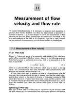
Fig. 12.2 Relationship between flow rate and stream function

a* a*
($),($),= (&I%) -l
(:I$)
=

x

This relationship shows that the streamline intersects normal to the
equipotential line at the crossing point of the two lines.
As shown in Fig. 12.2, consider points A and B on two closely
neighbouring streamlines, ) I and II/ d+. The volume flow rate dQ flowing in
unit time and crossing line AB is as follows from the figure:

+

a*

dQ = u dy - udx = -dy
ay

a*
+ -dX
ax

= d$

The volume flow rate Q of fluid flowing between two streamlines $ = $,
and $ = 9, is thus given by the following equation:

Q = TdQ = / y d $

=$
,

-IC/,

( 12.1 5)

I

Substituting eqn (12.12) into (4.8) for flow without vorticity, the following
is obtained, clarifying that the stream function satisfies Laplace’s equation:

-+,=o
$*
ax2

$*
ay

(12.16)

For a two-dimensional incompressible potential flow, since the velocity
potential Cp and stream function h exist, the following equations result from
,t
eqns (12.3) and (12.12):


202

Flow of

an ideal fluid
( 12.1 7)

These equations are called the Cauchy-Riemann equations in the theory of
complex variables. In this case they express the relationship between the
velocity potential and stream function. The Cauchy-Riemann equations
clarify the fact that 4 and $ both satisfy Laplace’s equation. They also clarify
the fact that a combination of 4 and t+b satisfying the Cauchy-Riemann
conditions expresses a two-dimensional incompressible potential flow.
Now, consider a regular function3 w(z) of complex variable z = x + iy and
express it as follows by dividing it into real and imaginary parts:

+

w(z) = 4 i$

z = x iy = r(cos e

+

*

4 = 44x3 Y
)

+ i sine) = rei6

( 12.18)

= *(x3 Y
)

and 4 and IC/ above satisfy eqn (12.17) owing to the nature of a regular
function. Consequently, real part 4(x, y) and imaginary part $(x, y) of the
regular function w(z) of complex number z can respectively be regarded as
the velocity potential and the stream function of the two-dimensional
incompressible potential flow. In other words, there exists an irrotational
motion whose equipotential line is $(x, y) = constant and streamline
$(x, y) = constant. Such a regular function w(z) is called the complex
potential.
From eqn (12.18)
aw
aw
dw=-dx+-dy=
ax
ay

= (u - iu)dx + (u

+ iu)dy = (u - iu)(dx + i dy) = (u - iu)dz

Therefore
dw
_ - -1u
-u
dz

(12.19)

Consequently, whenever w(z) is differentiated with respect to z, as shown
in Fig. 12.3, its real part yields velocity u in the x direction, and the negative
of its imaginary part yields velocity u in the y direction. The actual velocity
u io is called the complex velocity while u - iu in the above equation is the
conjugate complex velocity.

+

The function whose differential at any point with respect to z is independent of direction in
the z plane is called a regular function. A regular function satisfies the Cauchy-Riemann
equations.


Example of potential flow 203

Fig. 12.3 Complex velocity

12.5.1 Basic example

Parallel flow
For the uniform flow U shown in Fig. 12.4, from eqn (12.3)

u = 84 u
-=

v = - afp
=o

ax

aY

Therefore

afp
afp
dfp=-dX+-dy=
ax
aY
fp = u x

Fig. 12.4 Parallel flow

Udx


204 Flow of an ideal fluid

From eqn (12.12)

u = -a* u
=

a*

u=----

aY

ax

-0

Therefore

a*
a+
d4=-dX+-dy=
ax
ay
w(z) = 4

*

Udy

= UY

+ iJ/ = U(x + iy) = U z

(12.20)

The complex potential of parallel flow U in the x direction emerges as
w(z) = uz.
Furthermore, if the complex potential is given as w(z) = U z , the conjugate
complex velocity is
dw
-=u

(12.21)
dz
clarifying again that it expresses a uniform flow in the direction of the x
axis.

Source
As shown in Fig. 12.5, consider a case where fluid discharges from the origin
(point 0) at quantity q per unit time. Putting velocity in the radial direction
on a circle of radius r to u,, the discharge q per unit thickness is
q = 27crv, = constant

From eqns (12.7) and (12.22)

Fig. 12.5 Source

(12.22)


Example of potential flow 205

Also, from eqn (12.7),

Integrating d 4 in the above equation gives

4=-1

2L
7

(12.23)

ogr

Then, from eqns (12.13) and (12.22),

Therefore

*=--e

4
2n

(12.24)

Consequently, the complex potential is expressed by the following equation:
w =4

+ i$

4

= -(Iogr

271

4
+ id) = -Iog(rei8)
2n

4
= -1ogz

2n

(12.25)

From eqns (12.23) and (12.24) it is known that the equipotential lines are a
set of circles centred at the origin while the streamlines are a set of radial lines
radiating from the origin. Also, it is noted that the flow velocity u, is inversely
proportional to the distance r from the origin.
Whenever q > 0, fluid flows out evenly from the origin towards the
periphery. Such a point is called a source. Conversely, whenever q < 0, fluid
is absorbed evenly from the periphery. Such a point is called a sink. 141 is
called the strength of the source or sink.

Free vortex
In Fig. 12.6, fluid rotates around the origin with tangential velocity v, at
any given radius r. The circulation r is as follows from eqn (4.9):
2n

2n

ug

ds = u,r

J,

d0 = ~ K T U ,

The velocity potential 4 is

Therefore

r

4=-0
21
7

(12.26)

It emerges that uo is inversely proportional to the distance from the centre.
The stream function $ is


206 Flow of an ideal fluid

Fig. 12.6 Vortex

u8 -- - _ -a* - lar 2x2

Therefore

*

= --I

ur=-=o
a*

r a8

r

2.n
Consequently, the complex potential is

Ogr

(12.27)

r
iT
iT
w(z)=4+i$ = - ( 8 = i l o g r ) =
--(logr+i8)=
--logz
(12.28)
2.n
2.n

2n
For clockwise circulation, w(z) = (il-/2.n).
From eqns (12.26) and (12.17), it is known that the equipotential lines are
a group of radial straight lines passing through the origin whilst the flow lines
are a group of concentric circles centred on the origin. This flow appears in
Fig. 12.5 with broken lines representing streamlines and solid lines as equipotential lines. The circulation r is positive counterclockwise, and negative
clockwise.
This flow consists of rotary motion in concentric circles around the origin
with the velocity inversely proportional to the distance from the origin. Such
a flow is called a free vortex while the origin point itself is a point vortex.
The circulation is also called the strength of the vortex.
12.5.2 Synthesising of flows
When there are two regular functions w,(z) and wz(z), the function obtained
as their sum
(12.29)
w(z) = w,(z) + wz(z)


Example of potential flow 207

is also a regular function. If wI and w 2 represent the complex potentials of
two flows, another complex potential is obtained from their sum. By
combining two two-dimensional incompressible potential flows in such a
manner, another flow can be obtained.

Combining a source and a sink
Assume that, as shown in Fig. 12.7, the source q is at point A (z = -a) and
sink -q is at point B (z = a).
The complex potential wI at any point z due to the source whose strength
is q at point A is

w1 = -log(z
4

2n

+ a)

(12.30)

The complex potential w 2 at any point z due to the sink whose strength is q
is
wp = --log(z
4

2n

- a)

(12.31)

Because of the linearity of Laplace's equation the complex potential w of
the flow which is the combination of these two flows is
w = -[log(z
4
2n

+ a) - log(z - a)]

(12.32)

Now, from Fig. 12.7, since
z + a = r,eiel z - a = r2eie2

from eqn (12.32)
w = - logq
r'
r2
21(
7

+ i(0, - 0,))

Therefore

Fig. 12.7 Definition of variables for source A and sink B combination

(12.33)


208 Flow of an ideal fluid

4 = Qlog(;)
2n

(12.34)

4

(12.35)

$ = -2n
@I

- 62)

Assuming 4 = constant from the first equation, equipotential lines are
obtainable which are Appolonius circles for points A and B (a group of
circles whose ratios of distances from fixed points A and B are constant).
Taking $ = constant, streamlines are obtainable which are found to be
another set of circles whose vertical angles are the constant angle (e, - 6,) for
chord AB (Fig. 12.8).
Consider the case where a +. 0 in Fig. 12.8, under the condition of
aq = constant. Then from eqn (12.32),
w=-log
q
2n

~

(;::;:)-n[z

-2

a+-

-

:(:y ]

+-

;(:)3

-

+... =!!!!=E
nz

(12.36)

z

A flow given by the complex potential of eqn (12.36) is called a doublet,
while m = aq/n is its strength. The concept of a doublet is the extremity of a
source and a sink of equal strength approaching infinitesimally close to each
other whilst increasing their strength.
From eqn (12.36),
m
w=-=mx+1y

x - iy
xz+y2

Fig. 12.8 Flow due to the combination of source and sink

(12.37)


Example of potentialflow 209

Fig. 12.9 Doublet

mx
x2 y2
*=- my
x2 y2

cp=-

+
+

(12.38)
(12.39)

From these equations, as shown in Fig. 12.9, an equipotential line is a circle
whose centre is on the x axis whilst being tangential to the y axis, and a
streamline is a circle whose centre is on the y axis whilst being tangential to
the x axis.

Flow around a cylinder
Consider a circle of radius r,, centred at the origin in uniform parallel flows.
In general, by placing a number of sources and sinks in parallel flows, flows
around variously shaped bodies are obtainable. In this case, however, by
superimposing parallel flows onto the same doublet shown in Fig. 12.9, flows
around a circle are obtainable as follows.
From eqns (12.29) and (12.36) the complex potential when a doublet is in
uniform flows U is
w(z)=

( ;
:
)

uz+-= u z+-m
Z


210 Flow of an ideal fluid

Now, put m / U = r;, and
w(z)=

u

(z + -!
)

(12.40)

Decompose the above using the relationship z = r(cos 8 + i sin e), and
w(z) = u( r

+ $)cos 8 + i u ( r - $)sin 8

4 = u(r+$)coso

(12.41)

II/= U(r-$)sinO

(12.42)

Also, the conjugate complex velocity is
dw
dz

-= u - -

Uri

(12.43)

Z2

with stagnation points at z = f r o . The streamline passing the stagnation
point II/ = 0 is given by the following equation:
(r-$)sine=o
This streamline consists of the real axis and the circle of radius r,, centred at
the origin. By replacing this streamline with a solid surface, the flow around a
cylinder is obtained as shown in Fig. 12.10.
The tangential velocity of flow around a cylinder is, from eqn (12.41),

. 2-u( 1 +
!=

u '-rae

2)

Since r = r,, on the cylinder surface,
uo = -2U sin 8

Fig. 12.10 Flow around a cylinder

sin 6

(12.44)


Example of potential flow 2 11

Fig. 12.11 Definitions of v, and e

I

When the directions of 8 and vo are arranged as shown in Fig. 12.11, this
becomes
vo = 2U sin 8

(12.45)

The complex potential when there is clockwise circulation
cylinder is, as follows from eqns (12.28) and (12.40),
w(z)=

( :
)

u z+-

:

+-logz

r around

the

(1 2.46)

The flow in this case turns out as shown in Fig. 12.12. The tangential
velocity v; on the cylinder surface is as follows:

Fig. 12.12 Flow around a cylinder with circulation


2 12 Flow of an ideal fluid

v; = 2Usine+-

r

(12.47)

27cr0

A simple flow can be studied within the limitations of the z plane as in the
preceding section. For a complex flow, however, there may be some
established cases of useful mapping of a transformation to another plane.

For example, by transforming flow around a cylinder etc. through mapping
functions onto some other planes, such complex flows as the flow around a
wing, and between the blades of a pump, blower or turbine, can be
determined.
Assume that there is the relationship

5 =m

(12.48)

+

+

c

between two complex variables z = x iy and 5 = 5 ir], and that is the
regular function of z. Consider a mesh composed of x=constant and
y = constant on the z plane as shown in Fig. 12.13. That mesh transforms to
another mesh composed of 5 = constant and q = constant on the 5 plane. In
other words, the pattern on the z plane is different from the pattern on the
plane but they are related to each other.
Further, assume that, as shown in Fig. 12.14, point eo corresponds to point
zo and that the points corresponding to points z1 and z2 both minutely off zo
are and Then

c

el

c2.

z1

- z 0 - r leio1
-

el - c2 = R1eW
From eqn (12.48),

c

Fig. 12.13 Corresponding mesh on and zplanes

z 2 -- z 0--2e
-

io2

C2 - eo = ReiB2


Conformal mapping 2 13

Fig. 12.14 Conformal mapping

lim
zl-+zZ

e),_;,=

( ) (w)
s
ZI

-z
o

=

lim

ZI-'Z2

z2 - z
o

or
R,eiBI

R2e Z
i
B

r ,eisl

r2eio2

--- -

From the above, it turns out that

2=- 2
R
rl

e2-e, = p 2 - p l

R,

and the minute triangles on the z plane are
AZOZIZ,

o<

AiOili2

(12.49)

This shows that even though the pattern as a whole on the z plane may be
very different from that on the [ plane, their minute sections are similar and
equiangularly mapped. Such a manner of pattern mapping is called
conformal mapping, andf(z) is the mapping function.
Now, consider the mapping function
i=z+;

U2

@>0)

(12.50)

Substitute a circle of radius a on the z plane, z = ae", into eqn (12.50),

i= a(eio+ ~/e")= a(ei8+ e-io) = 2acos e
(12.5 1)
At the time when 8 changes from 0 to 2n, 5 corresponds in
2a + 0 + -2a + 0 + 2a. In other words, as shown in Fig. 12.15(a), the
cylinder on the z plane is conformally mapped onto the flat board on the i
plane. The mapping function in eqn (12.50) is renowned, and is called
Joukowski's transformation.
If conformal mapping is made onto the [ plane using Joukowski's mapping
function (12.50) while changing the position and size of a cylinder on the z
plane, the shape on the [ plane changes variously as shown in Fig. 12.15.


214 Flow of an ideal fluid

Fig. 12.15 Mapping of cylinders through Joukowski’s transformation: (a) flat plate; (b) elliptical
section; ( 3 symmetrical wing; (d) asymmetricalwing


Conformal mapping 2 15

The flow around the asymmetrical wing appearing in Fig. 12.15(d) can be
obtained by utilising Joukowski's conversion. Consider the flow in the case
where a cylinder of eccentricity zo and radius ro is placed in a uniform flow U
whose circulation strength is r. The complex potential of this flow can be
obtained by substituting z - zo for z in eqn (12.46),

(

w = u (z-zo)+-

"

z-zo

) + i 1log(z
21
7

- zo)

(12.52)

Putting z = zo + re", from w = Cp + i$

d = U(r+$)cose--e r
21
7

+ = U(r-$)sine--logr r
21t

(12.53)
(12.54)

On the circle r = r,, $ = constant, comprising a streamline. According to
the Kutta condition4 (where the trailing edge must become a stagnation

point),

r

2ur0 sina - - = o
271

@)o=-B=

(12.55)

r=rg

Therefore

r = 41tUrosinp

(12.56)

Fig. 12.16 Mapping of flow around cylinder onto flow around wing

4 If the trailing edge was not a stagnation point, the flow would go around the sharp edge at
infinite velocity from the lower face of the wing towards the upper face. The Kutta condition
avoids this physical impossibility.


2 16 Flow of an ideal fluid

Equipotential lines and streamlines produced by substituting values of r satisfying eqn (12.56) into eqns (12.53) and (12.54) are shown in Fig. 12.16(a).
They can be conformally mapped onto the [ plane by utilising Joukowski’s

conversion by eliminating z from eqns (12.50) and (12.52) to obtain the
complex potential on the [ plane. The resulting flow pattern around a wing
can be found as shown in Fig. 12.16(b). In this way, by means of conformal
mapping of simple flows, such as around a cylinder, flow around complexshaped bodies can be found.
Since the existence of analytical functions which shift z to the outside
territory of given wing shapes is generally known, the behaviour of flow
around these wings can be found from the flow around a cylinder through a
process similar to the previous one. In addition, there are examples where it
can be used for computing the contraction coefficient5of flow out of an orifice
in a large vessel and the drag6 due to the flow behind a flat plate normal to
the flow.

1. Obtain the velocity potential and the flow function for a flow whose
components of velocity in the x and y directions at a given point in the
flow are u,, and u,, respectively.

2. Show the existence of the following relationship between flow function
$ and the velocity components vr, ug in a two-dimensional flow:
vg=--

a*
ar

v=-

a*
rat2

3. What is the flow whose velocity potential is expressed as Cp = TO/2z?

4. Obtain the velocity potential and the stream function for radial flow
from the origin at quantity q per unit time.
5. Assuming that $ = U ( r - r i / r ) sin 8 expresses the stream function around
a cylinder of radius r,, in a uniform flow of velocity U, obtain the velocity
distribution and the pressure distribution on the cylinder surface.

6. Obtain the pattern of flow whose complex potential is expressed as
w = x 2.
7. What is the flow expressed by the following complex potential?

’ Lamb, H., Hydrodynamics, (1932), 6th edition, 98, Cambridge University Press.
Kirchhoff, G . , Grelles Journal, 70 (1 869), 289.


Problems 217

8. Obtain the complex potential of a uniform flow at angle c( to the x axis.

9. Obtain the streamline y = k and the equipotential line x = c of a flow
parallel to the x axis on the z plane when mapped onto the plane by
mapping function = l/z.

c

c

10. Obtain the flow in the case where parallel flow w = Uz on the z plane is
mapped onto the c plane by mapping function c = z1I3.