Financial economics a concise introduction to classical and behavioral finance

Financial Economics


•


Thorsten Hens

•

Marc Oliver Rieger

Financial Economics
A Concise Introduction
to Classical and Behavioral Finance

123


Professor Dr. Thorsten Hens
ISB, University of Zurich
Plattenstrasse 32
8032 Zurich
Switzerland


Prof. Dr. Marc Oliver Rieger
Fachbereich IV
University of Trier
Universitätsring 15

54286 Trier
Germany


ISBN 978-3-540-36146-6
e-ISBN 978-3-540-36148-0
DOI 10.1007/978-3-540-36148-0
Springer Heidelberg Dordrecht London New York
Library of Congress Control Number: 2010930284
c Springer-Verlag Berlin Heidelberg 2010
This work is subject to copyright. All rights are reserved, whether the whole or part of the material is
concerned, specifically the rights of translation, reprinting, reuse of illustrations, recitation, broadcasting,
reproduction on microfilm or in any other way, and storage in data banks. Duplication of this publication
or parts thereof is permitted only under the provisions of the German Copyright Law of September 9,
1965, in its current version, and permission for use must always be obtained from Springer. Violations are
liable to prosecution under the German Copyright Law.
The use of general descriptive names, registered names, trademarks, etc. in this publication does not imply,
even in the absence of a specific statement, that such names are exempt from the relevant protective laws
and regulations and therefore free for general use.
Cover design: WMX Design, GmbH
Printed on acid-free paper
Springer is part of Springer Science+Business Media (www.springer.com)


Preface

Until recently, most people were not paying too much attention to financial
markets. This certainly changed with the onset of the financial crisis. For a
long time we took it for granted that we can borrow money from a bank or get
safe interest payments on deposits. All these fundamental beliefs were shaken

in the wake of the financial crisis.
When the man on the street has lost his faith in systems which he believed
to function as steadily as the rotation of the earth, how much more have
the beliefs of financial economists been shattered? But the good news is: in
recent years, the theory of financial economics has incorporated many aspects
that now help to understand many of the bizarre market phenomena that
we could observe during the financial crisis. In the early days of financial
economics, the fundamental assumption was that markets are always efficient
and market participants perfectly rational. These assumptions allowed to build
an impressive theoretical model that was indeed useful to understand quite a
few characteristics of financial markets. Nevertheless, a major financial crisis
was not necessary to realize that the assumptions of perfectly efficient markets
with perfectly rational investors did not hold – often not even “on average”.
The observation of systematic deviations gave birth to a new theory, or rather
a set of new theories, behavioral finance theories.
While classical finance remains the cornerstone of financial theory – and be
it only as a benchmark that helps us to judge how much real markets deviate
from efficiency and rationality – behavioral finance enriches the view on the
real market and helps to explain many of the more detailed phenomena that
might be minor on sunny days, but decisive in rough weather.
Often, behavioral finance is introduced as something independent of financial economics. It is assumed that behavioral finance is something students
may learn after they have mastered and understood all of the classical financial
economics.
In this book we would like to follow a different approach. As market behavior can only be fully understood when behavioral effects are linked to classic
models, this book integrates both views from the very beginning. There is


VI

Preface

no separate chapter on behavioral finance in this book. Instead, all classic
topics (such as decisions on markets, the capital asset pricing model, market
equilibria etc.) are immediately connected with behavioral views. Thus, we
will never stay in a purely theoretical world, but look at the “real” one. This
is supported with many case studies on market phenomena, both during the
financial crisis and before.
How this book works and how it can be used for teaching or self-study is
explained in detail in the introduction (Chapter 1).
For now we would like to take the opportunity to thank all those people
who helped us write this book. First of all, we would like to thank many of our
colleagues for their valuable input, in particular Anke Gerber, Bjørn Sandvik,
Mei Wang, and Peter W¨
ohrmann.
Parts of this book are based on scripts and other teaching material that
was initially composed by former and present students of ours, in particular
by Berno B¨
uchel, Nil¨
ufer Caliskan, Christian Reichlin, Marc Sommer and
Andreas Tupak.
Many people contributed to the book by means of corrections or proofreading. We would like to thank especially Amelie Brune, Julia Buge, Marius Costeniuc, Michal Dzielinski, Mihnea Constantinescu, Mustafa Karama,
R. Vijay Krishna, Urs Schweri, Vedran Stankovic, Christoph Steikert, SvenChristian Steude, Laura Oehen and the best secretary of the world, Martine
Baumgartner.
That this book is not only an idea, but a real printed book with hundreds
of pages and thousands of formulas is entirely due to the fact that we had two
tremendously efficient LATEX professionals working for us. A big “thank you”
goes therefore to Thomas Rast and Eveline Hardmeier.
We also want to thank our publishers for their support, and especially
Martina Bihn for her patience in coping with the inevitable delays of finishing
this book.

Finally, we thank our families for their even larger patience with their
book-writing husbands and fathers.
We hope that you, dear reader, will have a good time with this book, and
that we can transmit some of our fascination for financial economics and its
interplay with behavioral finance to you.
Enjoy!
Thorsten Hens
Marc Oliver Rieger


Contents

Part I Foundations
1

Introduction . . . . . . . . . . . . . . . . . . . . . . . . . . . . . . . . . . . . . . . . . . . . . . .
1.1 An Introduction to This Book . . . . . . . . . . . . . . . . . . . . . . . . . . . . .
1.2 An Introduction to Financial Economics . . . . . . . . . . . . . . . . . . . .
1.2.1 Trade and Valuation in Financial Markets . . . . . . . . . . . .
1.2.2 No Arbitrage and No Excess Returns . . . . . . . . . . . . . . . .
1.2.3 Market Efficiency . . . . . . . . . . . . . . . . . . . . . . . . . . . . . . . . . .
1.2.4 Equilibrium . . . . . . . . . . . . . . . . . . . . . . . . . . . . . . . . . . . . . .
1.2.5 Aggregation and Comparative Statics . . . . . . . . . . . . . . . .
1.2.6 Time Scale of Investment Decisions . . . . . . . . . . . . . . . . . .
1.2.7 Behavioral Finance . . . . . . . . . . . . . . . . . . . . . . . . . . . . . . . .
1.3 An Introduction to the Research Methods . . . . . . . . . . . . . . . . . .

3
3
5

5
7
8
9
10
10
11
12

2

Decision Theory . . . . . . . . . . . . . . . . . . . . . . . . . . . . . . . . . . . . . . . . . . .
2.1 Fundamental Concepts . . . . . . . . . . . . . . . . . . . . . . . . . . . . . . . . . . .
2.2 Expected Utility Theory . . . . . . . . . . . . . . . . . . . . . . . . . . . . . . . . . .
2.2.1 Origins of Expected Utility Theory . . . . . . . . . . . . . . . . . .
2.2.2 Axiomatic Definition . . . . . . . . . . . . . . . . . . . . . . . . . . . . . . .
2.2.3 Which Utility Functions are “Suitable”? . . . . . . . . . . . . . .
2.2.4 Measuring the Utility Function . . . . . . . . . . . . . . . . . . . . . .
2.3 Mean-Variance Theory . . . . . . . . . . . . . . . . . . . . . . . . . . . . . . . . . . .
2.3.1 Definition and Fundamental Properties . . . . . . . . . . . . . . .
2.3.2 Success and Limitation . . . . . . . . . . . . . . . . . . . . . . . . . . . . .
2.4 Prospect Theory . . . . . . . . . . . . . . . . . . . . . . . . . . . . . . . . . . . . . . . .
2.4.1 Origins of Behavioral Decision Theory . . . . . . . . . . . . . . .
2.4.2 Original Prospect Theory . . . . . . . . . . . . . . . . . . . . . . . . . . .
2.4.3 Cumulative Prospect Theory . . . . . . . . . . . . . . . . . . . . . . . .
2.4.4 Choice of Value and Weighting Function . . . . . . . . . . . . .
2.4.5 Continuity in Decision Theories . . . . . . . . . . . . . . . . . . . .
2.4.6 Other Extensions of Prospect Theory . . . . . . . . . . . . . . .

15

16
20
20
28
36
43
47
47
48
52
53
56
60
67
71
73


VIII

Contents

2.5
2.6
2.7
2.8
2.9

Connecting EUT, Mean-Variance Theory and PT . . . . . . . . . . . .
Ambiguity and Uncertainty . . . . . . . . . . . . . . . . . . . . . . . . . . . . . .

Time Discounting . . . . . . . . . . . . . . . . . . . . . . . . . . . . . . . . . . . . . . .
Summary . . . . . . . . . . . . . . . . . . . . . . . . . . . . . . . . . . . . . . . . . . . . . . .
Tests and Exercises . . . . . . . . . . . . . . . . . . . . . . . . . . . . . . . . . . . . . .
2.9.1 Tests . . . . . . . . . . . . . . . . . . . . . . . . . . . . . . . . . . . . . . . . . . . .
2.9.2 Exercises . . . . . . . . . . . . . . . . . . . . . . . . . . . . . . . . . . . . . . . . .

75
80
82
85
86
86
89

Part II Financial Markets
3

Two-Period Model: Mean-Variance Approach . . . . . . . . . . . . . . 95
3.1 Geometric Intuition for the CAPM . . . . . . . . . . . . . . . . . . . . . . . . 96
3.1.1 Diversification . . . . . . . . . . . . . . . . . . . . . . . . . . . . . . . . . . . . 97
3.1.2 Efficient Frontier . . . . . . . . . . . . . . . . . . . . . . . . . . . . . . . . . . 99
3.1.3 Optimal Portfolio of Risky Assets with a Riskless
Security . . . . . . . . . . . . . . . . . . . . . . . . . . . . . . . . . . . . . . . . . . 99
3.1.4 Mathematical Analysis of the Minimum-Variance
Opportunity Set . . . . . . . . . . . . . . . . . . . . . . . . . . . . . . . . . . 100
3.1.5 Two-Fund Separation Theorem . . . . . . . . . . . . . . . . . . . . . 105
3.1.6 Computing the Tangent Portfolio . . . . . . . . . . . . . . . . . . . . 106
3.2 Market Equilibrium . . . . . . . . . . . . . . . . . . . . . . . . . . . . . . . . . . . . . . 107
3.2.1 Capital Asset Pricing Model . . . . . . . . . . . . . . . . . . . . . . . . 107
3.2.2 Application: Market Neutral Strategies . . . . . . . . . . . . . . . 108

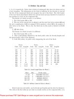
3.2.3 Empirical Validity of the CAPM . . . . . . . . . . . . . . . . . . . . 109
3.3 Heterogeneous Beliefs and the Alpha . . . . . . . . . . . . . . . . . . . . . . . 110
3.3.1 Definition of the Alpha . . . . . . . . . . . . . . . . . . . . . . . . . . . . . 112
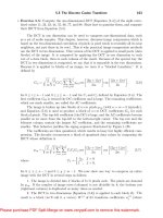
3.3.2 CAPM with Heterogeneous Beliefs . . . . . . . . . . . . . . . . . . . 116
3.3.3 Zero Sum Game . . . . . . . . . . . . . . . . . . . . . . . . . . . . . . . . . . . 120
3.3.4 Active or Passive? . . . . . . . . . . . . . . . . . . . . . . . . . . . . . . . . . 124
3.4 Alternative Betas and Higher Moment Betas . . . . . . . . . . . . . . . . 126
3.4.1 Alternative Betas . . . . . . . . . . . . . . . . . . . . . . . . . . . . . . . . . . 127
3.4.2 Higher Moment Betas . . . . . . . . . . . . . . . . . . . . . . . . . . . . . . 128
3.4.3 Deriving a Behavioral CAPM . . . . . . . . . . . . . . . . . . . . . . . 130
3.5 Summary . . . . . . . . . . . . . . . . . . . . . . . . . . . . . . . . . . . . . . . . . . . . . . . 135
3.6 Tests and Exercises . . . . . . . . . . . . . . . . . . . . . . . . . . . . . . . . . . . . . . 136
3.6.1 Tests . . . . . . . . . . . . . . . . . . . . . . . . . . . . . . . . . . . . . . . . . . . . 136
3.6.2 Exercises . . . . . . . . . . . . . . . . . . . . . . . . . . . . . . . . . . . . . . . . . 139

4

Two-Period Model: State-Preference Approach . . . . . . . . . . . . 141
4.1 Basic Two-Period Model . . . . . . . . . . . . . . . . . . . . . . . . . . . . . . . . . 141
4.1.1 Asset Classes . . . . . . . . . . . . . . . . . . . . . . . . . . . . . . . . . . . . . 142
4.1.2 Returns . . . . . . . . . . . . . . . . . . . . . . . . . . . . . . . . . . . . . . . . . . 143
4.1.3 Investors . . . . . . . . . . . . . . . . . . . . . . . . . . . . . . . . . . . . . . . . . 145
4.1.4 Complete and Incomplete Markets . . . . . . . . . . . . . . . . . . . 151
4.1.5 What Do Agents Trade? . . . . . . . . . . . . . . . . . . . . . . . . . . . 152


Contents

IX

4.2 No-Arbitrage Condition . . . . . . . . . . . . . . . . . . . . . . . . . . . . . . . . . . 152
4.2.1 Introduction . . . . . . . . . . . . . . . . . . . . . . . . . . . . . . . . . . . . . . 152
4.2.2 Fundamental Theorem of Asset Prices . . . . . . . . . . . . . . . 154
4.2.3 Pricing of Derivatives . . . . . . . . . . . . . . . . . . . . . . . . . . . . . . 160
4.2.4 Limits to Arbitrage . . . . . . . . . . . . . . . . . . . . . . . . . . . . . . . . 162
4.3 Financial Markets Equilibria . . . . . . . . . . . . . . . . . . . . . . . . . . . . . . 167
4.3.1 General Risk-Return Tradeoff . . . . . . . . . . . . . . . . . . . . . . . 168
4.3.2 Consumption Based CAPM . . . . . . . . . . . . . . . . . . . . . . . . . 169
4.3.3 Definition of Financial Markets Equilibria . . . . . . . . . . . . 170
4.3.4 Intertemporal Trade . . . . . . . . . . . . . . . . . . . . . . . . . . . . . . . 174
4.4 Special Cases: CAPM, APT and Behavioral CAPM . . . . . . . . . . 177
4.4.1 Deriving the CAPM by ‘Brutal Force
of Computations’ . . . . . . . . . . . . . . . . . . . . . . . . . . . . . . . . . . 178
4.4.2 Deriving the CAPM from the Likelihood
Ratio Process . . . . . . . . . . . . . . . . . . . . . . . . . . . . . . . . . . . . . 180
4.4.3 Arbitrage Pricing Theory . . . . . . . . . . . . . . . . . . . . . . . . . . . 182
4.4.4 Deriving the APT in the CAPM
with Background Risk . . . . . . . . . . . . . . . . . . . . . . . . . . . . . 183
4.4.5 Behavioral CAPM . . . . . . . . . . . . . . . . . . . . . . . . . . . . . . . . . 184
4.5 Pareto Efficiency . . . . . . . . . . . . . . . . . . . . . . . . . . . . . . . . . . . . . . . . 185
4.6 Aggregation . . . . . . . . . . . . . . . . . . . . . . . . . . . . . . . . . . . . . . . . . . . . 188
4.6.1 Anything Goes and the Limitations of Aggregation . . . . 188
4.6.2 A Model for Aggregation of Heterogeneous Beliefs,
Risk- and Time Preferences . . . . . . . . . . . . . . . . . . . . . . . . . 194
4.6.3 Empirical Properties of the Representative Agent . . . . . . 195
4.7 Dynamics and Stability of Equilibria . . . . . . . . . . . . . . . . . . . . . . . 201
4.8 Summary . . . . . . . . . . . . . . . . . . . . . . . . . . . . . . . . . . . . . . . . . . . . . . . 206
4.9 Tests and Exercises . . . . . . . . . . . . . . . . . . . . . . . . . . . . . . . . . . . . . . 207
4.9.1 Tests . . . . . . . . . . . . . . . . . . . . . . . . . . . . . . . . . . . . . . . . . . . . 207
4.9.2 Exercises . . . . . . . . . . . . . . . . . . . . . . . . . . . . . . . . . . . . . . . . . 209

5

Multiple-Periods Model . . . . . . . . . . . . . . . . . . . . . . . . . . . . . . . . . . . 221
5.1 The General Equilibrium Model . . . . . . . . . . . . . . . . . . . . . . . . . . . 221
5.2 Complete and Incomplete Markets . . . . . . . . . . . . . . . . . . . . . . . . . 226
5.3 Term Structure of Interest . . . . . . . . . . . . . . . . . . . . . . . . . . . . . . . . 228
5.3.1 Term Structure without Risk . . . . . . . . . . . . . . . . . . . . . . . 229
5.3.2 Term Structure with Risk . . . . . . . . . . . . . . . . . . . . . . . . . . 232
5.4 Arbitrage in the Multi-Period Model . . . . . . . . . . . . . . . . . . . . . . . 234
5.4.1 Fundamental Theorem of Asset Pricing . . . . . . . . . . . . . . 234
5.4.2 Consequences of No-Arbitrage . . . . . . . . . . . . . . . . . . . . . . 236
5.4.3 Applications to Option Pricing . . . . . . . . . . . . . . . . . . . . . . 236
5.4.4 Stock Prices as Discounted Expected Payoffs . . . . . . . . . . 238
5.4.5 Equivalent Formulations of the No-Arbitrage
Principle . . . . . . . . . . . . . . . . . . . . . . . . . . . . . . . . . . . . . . . . . 239
5.4.6 Ponzi Schemes and Bubbles . . . . . . . . . . . . . . . . . . . . . . . . . 240


X

Contents

5.5 Pareto Efficiency . . . . . . . . . . . . . . . . . . . . . . . . . . . . . . . . . . . . . . . . 244
5.5.1 First Welfare Theorem . . . . . . . . . . . . . . . . . . . . . . . . . . . . . 244
5.5.2 Aggregation . . . . . . . . . . . . . . . . . . . . . . . . . . . . . . . . . . . . . . 245
5.6 Dynamics of Price Expectations . . . . . . . . . . . . . . . . . . . . . . . . . . . 246
5.6.1 What is Momentum? . . . . . . . . . . . . . . . . . . . . . . . . . . . . . . 246
5.6.2 Dynamical Model of Chartists and Fundamentalists . . . . 247
5.7 Survival of the Fittest on Wall Street . . . . . . . . . . . . . . . . . . . . . . 252
5.7.1 Market Selection Hypothesis with Rational

Expectations . . . . . . . . . . . . . . . . . . . . . . . . . . . . . . . . . . . . . . 252
5.7.2 Evolutionary Portfolio Theory . . . . . . . . . . . . . . . . . . . . . . 253
5.7.3 Evolutionary Portfolio Model . . . . . . . . . . . . . . . . . . . . . . . 254
5.7.4 The Unique Survivor: λ . . . . . . . . . . . . . . . . . . . . . . . . . . . 258
5.8 Summary . . . . . . . . . . . . . . . . . . . . . . . . . . . . . . . . . . . . . . . . . . . . . . . 259
5.9 Tests and Exercises . . . . . . . . . . . . . . . . . . . . . . . . . . . . . . . . . . . . . . 259
5.9.1 Tests . . . . . . . . . . . . . . . . . . . . . . . . . . . . . . . . . . . . . . . . . . . . 259
5.9.2 Exercises . . . . . . . . . . . . . . . . . . . . . . . . . . . . . . . . . . . . . . . . . 260
Part III Advanced Topics
6

Theory of the Firm . . . . . . . . . . . . . . . . . . . . . . . . . . . . . . . . . . . . . . . 267
6.1 Basic Model . . . . . . . . . . . . . . . . . . . . . . . . . . . . . . . . . . . . . . . . . . . . 267
6.2 Modigliani-Miller Theorem . . . . . . . . . . . . . . . . . . . . . . . . . . . . . . . 274
6.2.1 When Does the Modigliani-Miller Theorem
Not Hold? . . . . . . . . . . . . . . . . . . . . . . . . . . . . . . . . . . . . . . . . 277
6.3 Firm’s Decision Rules . . . . . . . . . . . . . . . . . . . . . . . . . . . . . . . . . . . . 278
6.3.1 Fisher Separation Theorem . . . . . . . . . . . . . . . . . . . . . . . . . 278
6.3.2 The Theorem of Dr`eze . . . . . . . . . . . . . . . . . . . . . . . . . . . . . 282
6.4 Summary . . . . . . . . . . . . . . . . . . . . . . . . . . . . . . . . . . . . . . . . . . . . . . . 285

7

Information Asymmetries on Financial Markets . . . . . . . . . . 287
7.1 Information Revealed by Prices . . . . . . . . . . . . . . . . . . . . . . . . . . . 288
7.2 Information Revealed by Trade . . . . . . . . . . . . . . . . . . . . . . . . . . . . 290
7.3 Moral Hazard . . . . . . . . . . . . . . . . . . . . . . . . . . . . . . . . . . . . . . . . . . . 292
7.4 Adverse Selection . . . . . . . . . . . . . . . . . . . . . . . . . . . . . . . . . . . . . . . . 293
7.5 Summary . . . . . . . . . . . . . . . . . . . . . . . . . . . . . . . . . . . . . . . . . . . . . . . 295

8

Time-Continuous Model . . . . . . . . . . . . . . . . . . . . . . . . . . . . . . . . . . . 297
8.1 A Rough Path to the Black-Scholes Formula . . . . . . . . . . . . . . . . 298
8.2 Brownian Motion and It¯
o Processes . . . . . . . . . . . . . . . . . . . . . . . . 301
8.3 A Rigorous Path to the Black-Scholes Formula . . . . . . . . . . . . . . 304
8.3.1 Derivation of the Black-Scholes Formula
for Call Options . . . . . . . . . . . . . . . . . . . . . . . . . . . . . . . . . . . 304
8.3.2 Put-Call Parity . . . . . . . . . . . . . . . . . . . . . . . . . . . . . . . . . . . 307


Contents

XI

8.4
8.5
8.6
8.7
8.8

Exotic Options and the Monte Carlo Method . . . . . . . . . . . . . . . 308
Connections to the Multi-Period Model . . . . . . . . . . . . . . . . . . . . 310
Time-Continuity and the Mutual Fund Theorem . . . . . . . . . . . . 315
Market Equilibria in Continuous Time . . . . . . . . . . . . . . . . . . . . . 318
Limitations of the Black-Scholes Model and Extensions . . . . . . . 321
8.8.1 Volatility Smile and Other Unfriendly Effects . . . . . . . . . 321
8.8.2 Not Normal: Alternatives to Normally Distributed
Returns . . . . . . . . . . . . . . . . . . . . . . . . . . . . . . . . . . . . . . . . . . 322

8.8.3 Jumping Up and Down: L´evy Processes . . . . . . . . . . . . . . 327
8.8.4 Drifting Away: Heston and GARCH Models . . . . . . . . . . 329
8.9 Summary . . . . . . . . . . . . . . . . . . . . . . . . . . . . . . . . . . . . . . . . . . . . . . . 332

Appendices
Mathematics . . . . . . . . . . . . . . . . . . . . . . . . . . . . . . . . . . . . . . . . . . . . . . . . . . 335
A.1 Linear Algebra . . . . . . . . . . . . . . . . . . . . . . . . . . . . . . . . . . . . . . . . . . 335
A.2 Basic Notions of Statistics . . . . . . . . . . . . . . . . . . . . . . . . . . . . . . . . 338
A.3 Basics in Topology . . . . . . . . . . . . . . . . . . . . . . . . . . . . . . . . . . . . . . . 341
A.4 How to Use Probability Measures . . . . . . . . . . . . . . . . . . . . . . . . . . 343
A.5 Calculus, Fourier Transformations and Partial Differential
Equations . . . . . . . . . . . . . . . . . . . . . . . . . . . . . . . . . . . . . . . . . . . . . . 347
A.6 General Axioms for Expected Utility Theory . . . . . . . . . . . . . . . . 351
Solutions to Tests and Exercises . . . . . . . . . . . . . . . . . . . . . . . . . . . . . . . 355
References . . . . . . . . . . . . . . . . . . . . . . . . . . . . . . . . . . . . . . . . . . . . . . . . . . . . . 357
Index . . . . . . . . . . . . . . . . . . . . . . . . . . . . . . . . . . . . . . . . . . . . . . . . . . . . . . . . . . 367


Part I

Foundations



1
Introduction
“Advice is the only commodity on the market where the
supply always exceeds the demand.” Anonymous

This first chapter provides an overview on financial economics and how to

study it: you will learn how we have designed this textbook and how you
can use it efficiently; we will give you an overview of the essence of financial
economics and some of its central ideas; we will finally summarize how research
in financial economics is done, what methods are used and how they interact
with each other.
If you are new to the field of financial economics, we hope that at the end
of this introduction your appetite to learn more about it has been sufficiently
stimulated to enjoy reading the rest (or at least the main parts) of this book,
and maybe even to immerse yourself deeper in this fascinating research area. If
you are already working in this field, you can lean back and relax while reading
the introduction and then pick the topics of this book that are interesting to
you. Since financial economics is a very active area of research into which we
have incorporated a number of very recent results, be assured that you will
find something new as well.

1.1 An Introduction to This Book
This book integrates classical and behavioral approaches to financial economics and contains results that have been found only recently. It can serve
several aims:
•
•
•

as a textbook for a master or PhD course. Some parts can also be used on
an advanced bachelor level,
for self-study,
as a reference to various topics and as an overview on current results in
financial economics and behavioral finance.

In the following we want to give you some recommendations on how to use
this book as a textbook and for self-studying. Further information and sample

4

1 Introduction

slides that can be used for teaching this book are available on the book’s
homepage: http://www.financial-economics.de.
The book has three parts: the foundations part consists of this introduction
and a chapter on decision theory. The second part on financial markets builds
a sophisticated model of financial markets step by step and is also the core of
this book. Finally, the third part presents advanced topics that sketch some
of the connections between financial economics and other fields in finance. In
the first two parts, every chapter is accompanied by a number of exercises
and tests (solutions can be found in the appendix). Tests are included in
order to enable self-studying and as an assessment of the progress made in a
chapter. Exercises are meant to deepen the understanding by working with
the presented material.

Timecontinuous
Models
Chap. 8

Information
Asymmetries
Chap. 7

Theory of
the Firm
Chap. 6

Multi-period
Models
Chap. 5

More on Two-period
Models – Chaps. 4.3–4.7
Behavioral CAPM

General Two-period Model
Chaps. 4.1–4.2

Chap. 3.4
CAPM
Chaps.
3.1–3.3

Classical Decision Theory

Prospect
Theory

Ambiguity

Chaps. 2.4–2.5

Chap. 2.6

Chaps. 2.1–2.3, 2.7
Fig. 1.1. An overview on the interdependence of the chapters in this book. If you

want to build up your course on this book, be careful that the “bricks do not fall
down”!

The level of difficulty usually increases gradually within a chapter. Difficult parts not needed in the subsequent chapters are marked with an asterisk.
The content of this book provides enough study/teaching material for two
semesters. For a one-semester class there are therefore various possible routes.
A reasonable suggestion for a bachelor class could be to cover Chap. 1, excerpts of Chap. 2, Chaps. 3.1–3.2. They may be spiced with some applications.


1.2 An Introduction to Financial Economics

5

A one-semester master course could be based on Chap. 1, main ideas of
Chap. 2, Chaps. 3–4 and some parts of Chap. 5. A two-semester course could
follow the whole book in order of presentation. For a one-semester PhD course
for students who have already taken a class in financial economics, one could
choose some of the advanced topics (especially Chaps. 5–8) and provide necessary material from previous chapters as needed (e.g., the behavioral decision
theory from Chaps. 2.4–2.5). The interdependence of the chapters in this book
is illustrated in Fig. 1.1.

1.2 An Introduction to Financial Economics
Finance is composed of many different topics. These include public finance, international finance, corporate finance, derivatives, risk management, portfolio
theory, asset pricing, and financial economics.
Financial economics is the interface that connects finance to economics.
This means that different research questions, methods and languages meet,
which can be very fruitful, but also sometimes confusing. To mitigate the
confusion, we will present common topics from both points of view, the economics and the finance perspective. In doing so, we hope to reduce potential
misunderstandings and help to explore the synergies of the subfields.
Most topics in finance are in some way or the other connected to financial

economics. We will discuss several of these connections and the relation to
neighboring disciplines in detail, see Fig. 1.2.
Having located financial economics on the scientific map, we are now ready
to start our expedition by an overview of the key ideas and research methods.
The central point is hereby the transfer of the concept of trade from economics
(where tangible goods are traded) to the concept of valuation used in finance.
1.2.1 Trade and Valuation in Financial Markets
Financial economics is about trade among agents, trading in well functioning
financial markets. At first sight, agents trade interest bearing or dividends
paying assets (bonds or stocks) as well as derivatives thereof in financial markets. But from an economic perspective, on financial markets, agents trade
time, risks and beliefs. Of course, agents are heterogeneous, i.e., they have
different valuations of time, risks and beliefs. One of the main topics of financial economics is therefore the aggregation of those different valuations at a
market equilibrium into market prices for time, risks and beliefs.
For a long time, researchers believed that the aggregation approach would
be sufficient to describe financial markets. Recently, however, this classical
view has been challenged by new theories (behavioral and evolutionary finance) as well as by the emergence of new trading strategies (as implemented,
e.g., by hedge funds). One of the goals of this book is to describe to what degree these new views on financial markets can be integrated into the classical


6

1 Introduction

Fig. 1.2. Connections of financial economics with other subfields of finance and
other disciplines

concepts and how they give rise to new insights into financial economics. In
this way, we lay the foundations to understand practitioner’s buzz words like
“Alpha”, “Alternative Beta” and “Pure Alpha”.
What do we mean by saying that markets trade risks, time and beliefs? Let

us explain this idea with some examples. The trading of risks can be explained
easily if we look at commodities. For example, a farmer is naturally exposed
to the risk of falling prices, whereas a food company is exposed to the risk
of increasing prices. Using forwards, both can agree in advance on a price for
the commodity, and thus trade risk in a way that reduces both parties’ risks.
There are other situations where one party might not reduce its risk, but
is willing to buy the risk from another party for a certain price: hedge funds
and insurance companies, although very different in their risk appetite, both
work by this fundamental principle.
How to trade “time” on financial markets? Here the difference between
investment horizons plays a role. If I want to buy a house, I prefer to do this
rather earlier than later, since I get a benefit from owning the house. A bank
will lend me money and wants to be paid for that with a certain interest. The
same mechanism we can also find on financial markets when companies and
states issue bonds. Sometimes the loan issued by the bank is bundled and
sold as some of these now infamous CDOs that were at the epicenter of the
financial crisis.


1.2 An Introduction to Financial Economics

7

We can also trade “beliefs” on financial markets. In fact, this is likely to
be the most frequent reason to trade: two agents differ in their opinion about
certain assets. If Investor A believes Asset 1 to be more promising and Investor
B believes Asset 2 to be the better choice, then there is obviously some reason
for both to trade. Is there really? Well, from their perspectives there is, but
of course only one of them can be right, so contrary to the first two reasons
for a trade (risk and time), where both parties will profit, here only one of

them (the smarter or luckier) will profit. We will discuss the consequences of
this observation in a simple model as “the hunt for Alpha” in Chapter 3.3.
But in all of these cases what does limit the amount of trading? If trading
is good for both parties (or at least they believe so), why do they not trade
infinite amounts? In all cases, the reason is the decreasing marginal utility
of the agents: eventually, the benefit from more trades will be outweighed by
other factors. For instance, if agents trade because of different beliefs, they
will still have the same differences in beliefs after their trade but they won’t
trade unlimited amounts due to their decreasing marginal utility in the states.
1.2.2 No Arbitrage and No Excess Returns
Financial markets are complex, and moreover practitioners and researchers
tend to use the same word for different concepts, so sometimes these concepts get mixed-up. An example of this is the frequent confusion between
no-arbitrage and no gains for trades. An efficient financial market is arbitragefree. An arbitrage opportunity is a self-financing trading strategy that does
not incur losses but gives positive returns. Many researchers and practitioners
agree that arbitrage strategies are so rare that one can assume they do not
exist.
This simple idea has far-reaching conclusions for the valuation of derivatives. Derivatives are assets whose payoffs depend on the payoff of other assets,
the underlying, the assets from which the derivative is derived. In the simple
case where the payoff of the derivative can be duplicated by a portfolio of the
underlying and e.g., a risk-free asset, the price of the derivative must be the
same as the value of the duplicating portfolio. Why? Suppose the derivative’s
price is actually higher than the value of the duplicating portfolio. In that
case, one can build an arbitrage strategy by shorting the asset and hedging
the payoff by holding the duplicating portfolio. If the price of the derivative
were less than that of the duplicating portfolio, one would trade the other
way round. Hence the principle of no-arbitrage ties asset prices to each other.
As we will see later, the absence of arbitrage also implies nice mathematical
properties for asset prices which allow one to describe them by methods from
stochastics, for example by martingales.
Often, however, the term “arbitrage” is used for a likely, but uncertain

gain by an investment strategy. Now, forgetting about the motivations for
trading like risk sharing and different time preferences, many people believe


8

1 Introduction

that the only reason to trade on financial markets would be to gain more than
others, more precisely: to generate excess returns or “a positive Alpha”.
Given that efficient markets are arbitrage-free, it is often argued that therefore such gains are not possible and hence trading on a financial market is
useless: in any point of time the market has already incorporated all future
opportunities. Thus, instead of cleverly weighing the pros and cons of various
assets, one could also choose the assets at random, like in the famous monkey
test, where a monkey throws darts on the Wall Street Journal to pick stocks
and competes with investment professionals (see [Mal90]).
However, this point of view is wrong in two ways: first, it completely
ignores the two other reasons for trading on financial markets, namely risk
and time. Secondly, there is a distinction between an arbitrage-free market
and one without any further opportunities for gains from trade returns. An
efficient market, i.e. a market without any further gains from trade, must be
arbitrage-free since arbitrage opportunities certainly give gains from trades.
However, the converse is not true. Absence of arbitrage does not mean that
you should not try to position yourself on the markets reflecting on your
beliefs, time preferences and risk aversion.
Saying that investments could be chosen at random just because markets
are arbitrage-free is like saying that when you go shopping in a shop without
bargains, you can pick your goods at random. Just try to buy the ingredients
for a tasty dinner in this way, and you will discover that this is not true.
There is another way of looking at this problem: If you consider the return

distribution of your portfolio, forming asset allocations means to construct
the return distribution that is most suitable for you. One motive for this
may simply be controlling the risk of your initial portfolio, which could, e.g.,
be achieved by buying capital protection. Even though all possible portfolios
would be arbitrage-free, the precise choice nevertheless matters to you.
Before we conclude this extremely important section we should mention
how the notion of excess returns is related to the concepts of absence of
arbitrage and no gains from trade. An excess return is a return higher than
the risk-free rate. An excess return is usually no arbitrage opportunity since
it carries some risks. Does it indicate gains from trade? In other words, should
you buy assets that have excess returns? Whether you ought to buy or not
depends on your risk preference relative to the risk the asset carries. For
example, a positive alpha is an excess return that is attractive if your risk
preference is to avoid variance and if your beliefs coincide with the average
beliefs in the market. However, if one of these conditions is not met, an asset
with positive alpha may not be a good choice, as we will see later.
1.2.3 Market Efficiency
The word “efficiency” has a double meaning in financial economics. One meaning – put forward by Fama – is that markets are efficient if prices incorporate
all information. For example, paying analysts to research the opportunities


1.2 An Introduction to Financial Economics

9

and the risks of certain companies is worthless because the market has already priced the company reflecting all available information. To illustrate
this view consider Fama and a pedestrian walking on the street. The pedestrian spots a 100 Dollar Bill and wants to pick it up. Fama, however, stops
by saying if the 100 Dollar Bill were real, someone would have picked it up
before.
The second meaning of efficiency is that efficient markets do not have any

unexploited gains from trade. Thus the allocation obtained on efficient markets cannot be improved by raising the utility of one agent without lowering
the utility of some other agent. This notion of efficiency is called Paretoefficiency. Mostly, when we refer to “efficiency” in our book, we will mean
Pareto-efficiency.
1.2.4 Equilibrium
Economics is based on the idea of understanding markets from the interaction
of optimizing agents. In a competitive equilibrium all agents trade in such a
way as to achieve the most desirable consumption pattern, and market prices
are such that all markets clear, i.e., in all markets demand is equal to supply.
Obviously, in a competitive equilibrium there cannot be arbitrage opportunities since otherwise no agent would find an optimal action. Exploiting the
arbitrage more would drive the agent’s utility to infinity and he would like
to trade infinite amounts of the assets involved, which conflicts with market
clearing. Note that the notion of equilibrium puts more restrictions on asset
prices than mere no-arbitrage. Equilibrium prices reflect the relative scarcity
of consumption in different states, the agents’ beliefs of the occurrence of the
states and their risk preferences. Moreover, in a complete market, at equilibrium there are no further gains from trade.
As a final remark on equilibrium one should note that for one given initial
allocation there can be multiple equilibria. Which one is actually obtained may
be a matter of exogenous factors like market sentiment or conventions. For
example, stock returns could be high or low when the weather is extremely
nice. Supposing that every trader believes in high stock returns when the
weather is extremely nice, stock returns will turn out to be high because the
agents’ trades make this belief self-fulfilling. However it could also be the other
way round, i.e., low returns when the weather is extremely nice.
In a financial market equilibrium the agents’ beliefs determine the market
reality and the market reality confirms agents’ beliefs. In the words of George
Soros [Sor98, page xxiii]:
Financial markets attempt to predict a future that is contingent on
the decisions people make in the present. Instead of just passively
reflecting reality, financial markets are actively creating the reality
that they, in turn, reflect. There is a two way connection between

present decisions and the future events, which I call reflexivity.


10

1 Introduction

1.2.5 Aggregation and Comparative Statics
Do we really need to know all agents’ beliefs, risk attitudes and initial endowments in order to determine asset prices at equilibrium? The answer is
“No”, fortunately! If equilibrium prices are arbitrage-free then they can be
supported by a single decision problem in which one so-called “representative
agent” optimizes his utility supposing he had access to all endowments. The
equilibrium prices found in the competitive equilibrium can also be thought
of as prices that induce a representative agent to demand total endowments.
For this trick to be useful one then needs to understand how the individual
beliefs and risk attitudes aggregate into those of the representative agent. In
the case of complete markets such aggregation rules can be found.
A final warning on the use of the representative agent methodology is
in order. This method describes asset prices by some as-if decision problem.
Hence it is constructed given the knowledge of the asset prices. It is not able
to predict asset prices “out-of-sample”, e.g., after some exogenous shock to
the economy.
1.2.6 Time Scale of Investment Decisions
Investors differ in their time horizon, information processing and reaction
time. Day traders for example make many investment decisions per day requiring fast information processing. Their reaction time is only a few seconds.
Other investors have longer investment horizons (e.g., one or more years).
Their investment decisions do not have to be made “just in time”. A popular investment advice for investors with a longer investment horizon is: “Buy
stocks and take a good long (20 years) sleep”. Investors following this advice
are expected to have a different perception to stocks as Benartzi and Thaler
[BT95] make pretty clear with the following example:

Compare two investors, Nick who calculates the gains and losses in
his portfolio every day, and Dick who only looks at his portfolio once
per decade. Since, on a daily basis, stocks go down in value almost
as often as they go up, Nick’s loss aversion will make stocks appear
very unattractive to him. In contrast, loss aversion will not have much
effect on Dick’s perception of stocks since at ten year horizons stocks
offer only a small risk of losing money.
Particularly important for an investment decision is the perception of the
situation. In the words of a day trader, interviewed by the Wall Street Journal
[Mos98], the situation is like this:
Ninety percent of what we do is based on perception. It doesn’t matter
if that perception is right or wrong or real. It only matters that other
people in the market believe it. I may know it’s crazy, I may think
it’s wrong. But I lose my shirt by ignoring it. This business turns on
decisions made in seconds. If you wait a minute to reflect on things,


1.2 An Introduction to Financial Economics

11

you’re lost. I can’t afford to be five steps ahead of everybody else in
the market. That’s suicide.
Thus, intraday price movements reflect how the average investor perceives
incoming news. In the very long run price movements are determined by trends
in fundamental data – like earnings, dividend growth and cash flows. A famous observation called excess volatility first made by Shiller [Shi81] is that
stock prices fluctuate around the long term trend by more than economic
fundamentals indicate. How the short run aspects get washed out in the long
run, i.e., how aggregation of fluctuations over time can be modelled is rather
unclear.

In this course we will consider three time scales: The short run (intraday
market clearing of demand and supply orders), the medium run (monthly
equalization of expectations) and the long run (yearly wealth dynamics).
1.2.7 Behavioral Finance
A rational investor should follow expected utility theory. However, it is often
observed that agents do not behave according to this rational decision model.
Since it is often important to understand actual investment behavior, the
concepts of classical (rational) decision theory have often been replaced with
a more descriptive approach that is labeled as “behavioral decision theory”.
Its application to finance led to the emergence of “behavioral finance” as
a subdiscipline. Richard Thaler once nicely defined what behavioral finance
is all about [Tha93]:
Behavioral finance is simply open-minded finance. [...] Sometimes in
order to find a solution to an [financial] empirical puzzle it is necessary
to entertain the possibility that some of the agents in the economy
behave less than fully rational some of the time.
Whenever there is need to study deviations from perfectly rational behavior,
we are already in the realm of behavioral finance. It is therefore quite obvious
that a clear distinction of problems inside and outside behavioral finance is
impossible: we will often be in situations where agents behave mostly rational, but not always, so that a simple model might be successful with only
considering rational behavior, but behavioral “corrections” have to be made
as soon as we take a closer look.
In this book we therefore aim to integrate behavioral views into classical
theories to show how they can enhance our understanding of financial markets.
One particularly interesting behavioral model is Prospect Theory. It was
developed by Daniel Kahneman and Amos Tversky [KT79] to describe decisions between risky alternatives. Prospect Theory departs from expected
utility by showing the sensitivity of actual decisions to biases like framing, by
using a valuation function that is defined on gains and losses instead of final
wealth and by using non-linear probability when weighting the utility values

12

1 Introduction

obtained in various states. In particular Prospect Theory investors are loss
averse, and they are risk averse when comparing two gains but risk seeking
when comparing two losses. The question then is whether Prospect Theory is
relevant for market prices. And indeed it is: many so-called asset pricing puzzles can be resolved with Prospect Theory. An example is the equity premium
puzzle, i.e., the observation that stock returns are on average 6–7% above
the bond returns. This high excess return is hard to explain with plausible
values for risk aversion, if one sticks to the expected utility paradigm. The
idea of myopic loss aversion (Benartzi and Thaler [BT95]), the observation
that investors have short horizons and are loss averse, can resolve the equity
premium puzzle.

1.3 An Introduction to the Research Methods
We want to conclude this chapter by taking a look at the research methods
that are used in financial economics. After all, we want to know where the
results we are studying come from and how we can possibly add new results.
Albert Einstein is known to have said that “there is nothing more practical
than a good theory.” But what is a good theory? First of all, a good theory
is based on observable assumptions. Moreover, a good theory should have
testable implications – otherwise it is a religion which cannot be falsified.
This falsification aspect cannot be stressed enough.1 Finally, a good theory
is a broad generalization of reality that captures its essential features. Note
that a theory does not become better if it becomes more complicated.
But what are our observations and implications? There are essentially two
ways to gather empirical evidence to support (or falsify) a theory on financial
markets: one way is to study financial market data. Some of this data (e.g.,

stock prices) is readily available, some is difficult to obtain for reasons such
as privacy issues or time constraints. The second way is to conduct surveys
and laboratory experiments, i.e., to expose subjects to controlled conditions
under which they have to perform financial decisions.
Both approaches have their advantages and limitations: market data is
often noisy, depends on many uncontrollable factors and might not be available
for a specific purpose, but by definition always comes from real life situations.
Experimental data often suffers from a small number of subjects, necessarily
unrealistic settings, but can be collected under controlled conditions. Today,
both methods are frequently used together (typically, experiments for the
more fundamental questions, like decision theory, and data analysis for more
1

Steve Ross, the founder of the econometric Arbitrage Pricing Theory (APT ), for
example, claims that “every financial disaster begins with a theory!” By saying
this, he means that those who start trading based on a theory are less likely
to react to disturbing facts because they are typically in love with their ideas.
Falsification of their beloved theory is certainly not their goal!


1.3 An Introduction to the Research Methods

13

applied questions, like asset pricing), and we will see many applications of
these approaches throughout this book.
So, what is a typical route that research in financial economics is taking?
Often a research question is born by looking at data and finding empirically
robust deviations from random behavior of asset prices. The next step is then
to try to explain these effects with testable hypotheses. Such hypotheses can

rely on classical concepts or on behavioral or evolutionary approaches. In the
latter cases, laboratory tests have often been performed first in order to test
these approaches under controlled conditions.
The role of empirical findings and its interplay with theoretical research
in finance cannot be overstressed. To quote Hal Varian[Var93b]:
Financial economics has been so successful because of this fruitful
relationship between theory and data. Many of the same people who
formulated the theories also collected and analyzed the data. This is
a model that the rest of the economic profession would do well to
emulate.
In any case, if you want to discover interesting effects in the stock market,
the main requirement is that you understand the “Null Hypothesis”. In this
case, it is what a rational market looks like. Therefore a big part of this book
will deal with traditional finance that explains the rational point of view.
We have now concluded our bird’s-eye view on financial economics and
on the contents of this book. Before we dive into financial markets with their
manifold interactions, we start with a more basic situation: in the next chapter
we will study the individual decisions a person makes with financial problems.
This leads us to the general field of decision theory which will later serve us
as a building block for the understanding of more complex interactions on the
market that involve not only one, but many persons.