Finite time exergoeconomic performance optimization for an irreversible universal steady flow variable-temperature heat reservoir heat pump cycle model

INTERNATIONAL JOURNAL OF

ENERGY AND ENVIRONMENT
Volume 1, Issue 6, 2010 pp.969-986
Journal homepage: www.IJEE.IEEFoundation.org

Finite time exergoeconomic performance optimization for
an irreversible universal steady flow variable-temperature
heat reservoir heat pump cycle model
Huijun Feng, Lingen Chen, Fengrui Sun
Postgraduate School, Naval University of Engineering, Wuhan 430033, P. R. China.

Abstract
An irreversible universal steady flow heat pump cycle model with variable-temperature heat reservoirs
and the losses of heat-resistance and internal irreversibility is established by using the theory of finite
time thermodynamics. The universal heat pump cycle model consists of two heat-absorbing branches,
two heat-releasing branches and two adiabatic branches. Expressions of heating load, coefficient of
performance (COP) and profit rate of the universal heat pump cycle model are derived, respectively. By
means of numerical calculations, heat conductance distributions between hot- and cold-side heat
exchangers are optimized by taking the maximum profit rate as objective. There exist an optimal heat
conductance distribution and an optimal thermal capacity rate matching between the working fluid and
heat reservoirs which lead to a double maximum profit rate. The effects of internal irreversibility, total
heat exchanger inventory, thermal capacity rate of the working fluid and heat capacity ratio of the heat
reservoirs on the optimal finite time exergoeconomic performance of the cycle are discussed in detail.
The results obtained herein include the optimal finite time exergoeconomic performances of
endoreversible and irreversible, constant- and variable-temperature heat reservoir Brayton, Otto, Diesel,
Atkinson, Dual, Miller and Carnot heat pump cycles.
Copyright © 2010 International Energy and Environment Foundation - All rights reserved.
Keywords: Finite time thermodynamics, Heating load, COP, Profit rate, Irreversible universal heat
pump cycle, Internal irreversibility, Optimal heat capacity rate matching, Exergoeconomic performance.

1. Introduction
Finite time thermodynamics (FTT) [1-15] has been a powerful tool for the performance analyses and
optimizations of various thermodynamic processes and cycles. The performance index in the analyses
and optimizations are often pure thermodynamic parameters, which include power output, efficiency,
entropy production rate, cooling load, heating load, coefficient of performance (COP), exergy loss, etc.
Exergoeconomic (or thermoeconomic) analysis [16, 17] is a relatively new method that combines exergy
with conventional concepts from long-run engineering economic optimization to evaluate and optimize
the design and performance of energy systems. Salamon and Nitzan’s work [18] combined the
endoreversible model in finite time thermodynamics with exergoeconomic analysis. It was termed as
finite time exergoeconomic analysis [19-36] to distinguish it from the endoreversible analysis with pure
thermodynamic objectives and the exergoeconomic analysis with long-run economic optimization. This
ideal has been extended to endoreversible [19-24] and generalized irreversible [25-27] Carnot heat
engines, refrigerators and heat pumps, universal steady flow two-heat-reservoir heat engine, refrigerator
ISSN 2076-2895 (Print), ISSN 2076-2909 (Online) ©2010 International Energy & Environment Foundation. All rights reserved.


970

International Journal of Energy and Environment (IJEE), Volume 1, Issue 6, 2010, pp.969-986

and heat pump cycles [28-31], three-heat-reservoir refrigerator and heat pump cycles [32, 33],
endoreversible and irreversible four-heat-reservoir absorption refrigerator [34], as well as endoreversible
closed-cycle simple and regenerative gas turbine heat and power cogeneration plants [35, 36]. In
succession, a new thermoeconomic optimization criterion, thermodynamic output rates (power, cooling
load or heating load for heat engine, refrigerator or heat pump) per unit total cost, was put forward by
Sahin and Kodal [37-41]. It was used to analyze and optimize the performances of endoreversible [37,
38] and irreversible [39, 40] Carnot heat engines [37, 39], refrigerators and heat pumps [38, 40], and
three-heat-reservoir absorption refrigerator and heat pump [41].
Generalization and unified description of thermodynamic cycle model is an important task of FTT
research. Finite time exergoeconomic optimization for endoreversible [30] and irreversible [31] universal

steady flow heat pump cycles with constant-temperature heat reservoirs have been studied, but practical
heat pump cycles are always irreversible ones and with variable-temperature heat reservoirs. There are
lacks of unified descriptions of exergoeconomic performances for various heat pump cycles with
variable-temperature heat reservoirs. On the basis of variable-temperature heat reservoir Carnot and
Brayton heat pump cycle models [42-45], this paper will build an irreversible universal steady flow heat
pump cycle model consisting of two heat-absorbing branches, two heat-releasing branches and two
adiabatic branches with variable-temperature heat reservoirs and the losses of heat-resistance and internal
irreversibility. The major work of this paper is to provide a unified description of the finite time
exergoeconomic performance for various irreversible heat pump cycles with variable-temperature heat
reservoirs. The results obtained herein include the optimal finite time exergoeconomic performance
characteristics of end reversible and irreversible variable- and constant-temperature heat reservoir
Brayton, Otto, Diesel, Atkinson, Dual, Miller and Carnot heat pump cycles.
2. Cycle model
An irreversible universal variable-temperature heat reservoir heat pump cycle model with heat-resistance
and internal irreversibility is shown in Figure 1. The following assumptions are made for this model:
(1) The working fluid is an ideal gas and flows through the system in a quasi-steady fashion. The cycle
consists of two heat-absorbing branches (1-2 and 2-3) with constant working fluid thermal capacity rates
(mass flow rate of the working fluid and specific heat product) Cwf 1 and Cwf 2 , two heat-releasing
branches (4-5 and 5-6) with constant working fluid thermal capacity rates Cwf 4 and Cwf 3 and two
adiabatic branches (3-4 and 6-1). All six processes are irreversible.
(2) The hot- and cold-side heat exchangers are considered to be counter-flow heat exchangers, the
working fluid temperatures are different from the heat reservoir temperatures owing to the heat transfer.
The heat transfer rate ( QH ) released to the heat sink, i.e. the heating load of the cycle, and the heat
transfer rate ( QL ) supplied by the heat source are:

QH = QH 1 + QH 2

(1)

QL = QL1 + QL 2

(2)

where QH 1 + QH 2 is due to the driving force of temperature differences between the high-temperature
(hot-side) heat sink and working fluid, QL1 + QL 2 is due to the driving force of temperature differences
between the low-temperature (cold-side) heat source and working fluid. The high-temperature heat sink
is considered with thermal capacity rate CH and the inlet and outlet temperatures of the heat-releasing
fluid are THin , THout1 and THout 2 , respectively. The low-temperature heat source is considered with thermal
capacity rate CL and the inlet and outlet temperatures of the heat-absorbing fluid are TLin , TLout1 and
TLout 2 , respectively.
(3) A constant coefficient φ is introduced to characterize the additional internal miscellaneous
'
'
irreversibility effects: φ = (QH 1 + QH 2 ) / (QH 1 + QH 2 ) ≥ 1 , where QH 1 + QH 2 is the rate of heat-flow from the
'
'
warm working-fluid to the heat-sink for the irreversible cycle model, while QH 1 + QH 2 is that for the
endoreversible cycle model with the only loss of heat-resistance.

ISSN 2076-2895 (Print), ISSN 2076-2909 (Online) ©2010 International Energy & Environment Foundation. All rights reserved.


International Journal of Energy and Environment (IJEE), Volume 1, Issue 6, 2010, pp.969-986

971

To summarize, the irreversible universal heat pump cycle model with variable-temperature heat
reservoirs is characterized by the following three aspects:
(1) The different values of CH and CL . If CH → ∞ and CL → ∞ , the cycle model is reduced to the
irreversible universal heat pump cycle model with constant-temperature heat reservoirs [31].

(2) The different values of Cwf 1 , Cwf 2 , Cwf 3 and Cwf 4 . If Cwf 1 , Cwf 2 , Cwf 3 and Cwf 4 have different values,
the cycle model can be reduced to various special heat pump cycles.
(3) The different values of φ . If φ = 1 , the cycle model is reduced to the endoreversible universal heat
pump cycle model with variable-temperature heat reservoirs. If φ = 1 , CH → ∞ and CL → ∞ further, the
cycle model is reduced to the endoreversible universal heat pump cycle model with constant-temperature
heat reservoirs [30].

Figure 1. Cycle model
According to the properties of heat transfer, heat reservoir, working fluid, and the theory of heat
exchangers, the heat transfer rates ( QH 1 and QH 2 ) released to the heat sink and the heat transfer rates ( QL1
and QL 2 ) supplied by heat source are, respectively, given by
QH 1 = U H 1[(T5 − THout1 ) − (T6 − THin )] / ln[(T5 − THout1 ) / (T6 − THin )] = CH (THout1 − THin )
= Cwf 3 (T5 − T6 ) = CH 1min EH 1 (T5 − THin )
QH 2 = U H 2 [(T4 − THout 2 ) − (T5 − THout1 )] / ln[(T4 − THout 2 ) / (T5 − THout1 )] = C H (THout 2 − THout1 )
= Cwf 4 (T4 − T5 ) = C H 2 min EH 2 (T4 − THout1 )
QL1 = U L1[(TLout1 − T2 ) − (TLout 2 − T1 )] / ln[(TLout1 − T2 ) / (TLout 2 − T1 )] = CL (TLout1 − TLout 2 )
= Cwf 1 (T2 − T1 ) = CL1min EL1 (TLout1 − T1 )

QL 2 = U L 2 [(TLin − T3 ) − (TLout1 − T2 )] / ln[(TLin − T3 ) / (TLout1 − T2 )] = CL (TLin − TLout1 )
= Cwf 2 (T3 − T2 ) = CL 2 min EL 2 (TLin − T2 )

(3)

(4)

(5)

(6)

where EH 1 , EH 2 , EL1 and EL 2 are the effectivenesses of the hot- and cold-side heat exchangers, and are

defined as:
EH 1 = {1 − exp[− N H 1 (1 − CH 1min / CH 1max )]} / {1 − (CH 1min / CH 1max ) exp[− N H 1 (1 − CH 1min / CH 1max )]}

(7)

ISSN 2076-2895 (Print), ISSN 2076-2909 (Online) ©2010 International Energy & Environment Foundation. All rights reserved.


International Journal of Energy and Environment (IJEE), Volume 1, Issue 6, 2010, pp.969-986

972

EH 2 = {1 − exp[− N H 2 (1 − CH 2 min / CH 2 max )]} / {1 − (CH 2 min / CH 2 max ) exp[− N H 2 (1 − CH 2 min / CH 2 max )]}

(8)

EL1 = {1 − exp[− N L1 (1 − CL1min / CL1max )]} / {1 − (CL1min / CL1max ) exp[− N L1 (1 − CL1min / CL1max )]}

(9)

EL 2 = {1 − exp[− N L 2 (1 − CL 2 min / CL 2 max )]} / {1 − (CL 2 min / CL 2 max ) exp[− N L 2 (1 − CL 2 min / CL 2 max )]}

(10)

where CH 1min and CH 1max are the minimum and maximum of CH and Cwf 3 , respectively; CH 2 min and
CH 2 max are the minimum and maximum of CH and Cwf 4 , respectively; CL1min and CL1max are the minimum
and maximum of CL and Cwf 1 , respectively; CL 2 min and CL 2 max are the minimum and maximum of CL
and Cwf 2 , respectively; and N H 1 , N H 2 , N L1 and N L 2 are the numbers of heat transfer units of the hot- and
cold-side heat exchangers, respectively:
CH 1min = min{CH , Cwf 3 } , CH 1max = max{CH , Cwf 3 }

(11)

CH 2 min = min{CH , Cwf 4 } , CH 2 max = max{CH , Cwf 4 }

(12)

CL1min = min{CL , Cwf 1} , CL1max = max{CL , Cwf 1}

(13)

CL 2 min = min{CL , Cwf 2 } , CL 2 max = max{CL , Cwf 2 }

(14)

N H 1 = U H 1 / CH 1min , N H 2 = U H 2 / CH 2 min , N L1 = U L1 / CL1min , N L 2 = U L 2 / CL 2 min

(15)

where U H 1 , U H 2 , U L1 and U L 2 are the heat conductances, that is, the product of heat transfer coefficient
α and heat transfer surface area F .
3. Finite time exergoeconomic performance analysis
Combining equations (3)-(6), one can obtain:
T5 = ( Cwf 3T6 − C H 1min EH 1THin ) ( Cwf 3 − C H 1min EH 1 )

T4 = [CH 1min CH 2 min Cwf 3 E H 1E H 2 (−T6 + THin ) / CH + CH 1min E H 1THin (−Cwf 4 + CH 2 min E H 2 ) +
Cwf 3 (Cwf 4T6 − CH 2 min E H 2THin )] [(Cwf 3 − CH 1min E H 1 )(Cwf 4 − CH 2 min E H 2 )]
T1 = [CL1min CL 2 min Cwf 2 E L1E L 2 (TLin − T3 ) CL + CL1min E L1TLin (CL 2 min E L 2 − Cwf 2 ) +
Cwf 1 (Cwf 2T3 − CL 2 min E L 2TLin )] / [(Cwf 1 − CL1min E L1 )(Cwf 2 − CL 2 min E L 2 )]
T2 = ( Cwf 2T3 − C L 2 min EL 2TLin ) ( Cwf 2 − C L 2 min EL 2 )

(16)

(17)

(18)

(19)

The second law of thermodynamics requires that:
'
'
φ = (QH 1 + QH 2 ) (QH 1 + QH 2 ) = (Cwf 3 ln

T5
T
T
T
+ Cwf 4 ln 4 ) (Cwf 1 ln 2 + Cwf 2 ln 3 )
T6
T5
T1
T2

(20)

Thus:

T2 = T1G

(21)

where:

ISSN 2076-2895 (Print), ISSN 2076-2909 (Online) ©2010 International Energy & Environment Foundation. All rights reserved.


International Journal of Energy and Environment (IJEE), Volume 1, Issue 6, 2010, pp.969-986
Cwf 3

G=x

φ Cwf 1

−

y

973

Cwf 2
Cwf 1
Cwf 4

⎧[CH 1min CH 2 min Cwf 3 E H 1E H 2 (−T6 + THin ) / CH + CH 1min E H 1THin (−Cwf 4 + CH 2 min E H 2 ) + ⎫φ Cwf 1
⎪
⎪
⎨
⎬
Cwf 3 (Cwf 4T6 − CH 2 min E H 2THin )] [(Cwf 3T6 − CH 1min EH 1THin )(Cwf 2 − CH 2 min E H 2 )] ⎪

⎪
⎩
⎭

(22)

where x = T5 T6 and y = T3 T2 .
Combining equations (3)-(6) with equations (18)-(22) gives:
T1 =

T2 =

T3 =

CL1min E L1TLin [CL 2 min Cwf 2 E L 2 + CL (−Cwf 2 + CL 2 min E L 2 )]
GyCL1min CL 2 min Cwf 2 E L1E L 2 − CL [Cwf 1 (G − 1) + CL1min E L1 ](Cwf 2 − CL 2 min E L 2 )
GCL1min E L1TLin [CL 2 min Cwf 2 E L 2 + CL (−Cwf 2 + CL 2 min E L 2 )]
GyCL1min CL 2 min Cwf 2 E L1E L 2 − CL [Cwf 1 (G − 1) + CL1min E L1 ](Cwf 2 − CL 2 min E L 2 )
GyCL1min E L1TLin [CL 2 min Cwf 2 E L 2 + CL (−Cwf 2 + CL 2 min E L 2 )]
GyCL1min CL 2 min Cwf 2 E L1E L 2 − CL [Cwf 1 (G − 1) + CL1min E L1 ](Cwf 2 − CL 2 min E L 2 )

(23)

(24)

(25)

2
THout 2 = [CH THin (Cwf 3 − CH 1min E H 1 )(Cwf 4 − CH 2 min E H 2 ) + CH 1min CH 2 min Cwf 3Cwf 4 E H 1 E H 2 ( −T6 + THin ) +

CH Cwf 3 (T6 − THin )(CH 2 min Cwf 4 E H 2 + CH 1min E H 1Cwf 4 − CH 1min CH 2 min E H 1 E H 2 ) ] /

(26)

[C (Cwf 3 − CH 1min E H 1 )(Cwf 4 − CH 2 min E H 2 )]
2
H

TLout 2 = {CL1min CL 2 min Cwf 1Cwf 2 E L1E L 2TLin [(G − 1)Cwf 1 + (1 − Gy )CL1min E L1 ] +
2
CL TLin (Cwf 1 − CL1min E L1 )(Cwf 1G + CL1min E L1 − Cwf 1 )(Cwf 2 − CL 2 min E L 2 ) +
2
2
2
CL Cwf 2TLin [(1 − G )CL 2 min Cwf 1E L 2 + CL1min E L1 (Cwf 1Gy + CL 2 min E L 2 − Cwf 1 ) +

(1 − G )Cwf 1CL1min Cwf 1E L1 + (G − 2)CL 2 min E L 2 CL1min Cwf 1E L1 ]} /

(27)

{(Cwf 1CL − CL1min CL E L1 )[−GyCL1min CL 2 min Cwf 2 E L1E L 2 +
CL (Cwf 1G + CL1min E L1 − Cwf 1 )(Cwf 2 − CL 2 min E L 2 )]}

Substituting equations (3), (4), (16) and (17) into equation (1) yields the heating load of the cycle:
QH = QH 1 + QH 2
= [−CH 1min CH 2 min Cwf 3Cwf 4 E H 1E H 2 (T6 − THin ) / CH + CH 2 min Cwf 3Cwf 4 E H 2 (T6 − THin ) +

(28)

CH 1min E H 1Cwf 3 (T6 − THin )(Cwf 4 − CH 2 min E H 2 )] / [(Cwf 3 − CH 1min E H 1 )(Cwf 4 − CH 2 min E H 2 )]

Substituting equations (5), (6), (18) and (19) into equation (2) yields the heat transfer rate supplied by the
heat source:
QL = QL1 + QL 2
2
2
= TLin {CL 2 min E L 2 (1 − CL1min E L1 / CL )[−G ( y − 1)CL1min Cwf 2 E L1 / CL − (G − 1)(Cwf 1 − CL1min E L1 )] +

CL 2 min E L 2 [CL1min Cwf 2 E L1 (Cwf 1 + CL1min E L1G − CL1min E L1Gy − Cwf 1G ) / CL +

(29)

(G − 1)(Cwf 1Cwf 2 − Cwf 1CL1min E L1 − Cwf 2 CL1min E L1 )] + (G − 1)CL1min Cwf 1Cwf 2 E L1}/
[(Cwf 1G + CL1min E L1 − Cwf 1 )(Cwf 2 − CL 2 min E L 2 ) − GyCL1min CL 2 min Cwf 2 E L1E L 2 / CL ]

Combining equations (28) with (29) gives the COP of the cycle:

ISSN 2076-2895 (Print), ISSN 2076-2909 (Online) ©2010 International Energy & Environment Foundation. All rights reserved.


International Journal of Energy and Environment (IJEE), Volume 1, Issue 6, 2010, pp.969-986

974
β=

QH
QH
=
P
QH − QL

[−CH 1min CH 2 min Cwf 3Cwf 4 E H 1E H 2 (T6 − THin ) / CH + CH 2 min Cwf 3Cwf 4 E H 2 (T6 − THin ) +
CH 1min E H 1Cwf 3 (T6 − THin )(Cwf 4 − CH 2 min E H 2 )] / [(Cwf 3 − CH 1min E H 1 )(Cwf 4 − CH 2 min E H 2 )]

=

[−CH 1min CH 2 min Cwf 3Cwf 4 E H 1E H 2 (T6 − THin ) / CH + CH 2 min Cwf 3Cwf 4 E H 2 (T6 − THin ) +
CH 1min E H 1Cwf 3 (T6 − THin )(Cwf 4 − CH 2 min E H 2 )] / [(Cwf 3 − CH 1min E H 1 )(Cwf 4 − CH 2 min E H 2 )] −

(30)

2
2
TLin {CL 2 min E L 2 (1 − CL1min E L1 / CL )[−G ( y − 1)CL1min Cwf 2 E L1 / CL − (G − 1)(Cwf 1 − CL1min E L1 )] +

CL 2 min E L 2 [CL1min Cwf 2 E L1 (Cwf 1 + CL1min E L1G − CL1min E L1Gy − Cwf 1G ) / CL +
(G − 1)(Cwf 1Cwf 2 − Cwf 1CL1min E L1 − Cwf 2 CL1min E L1 )] + (G − 1)CL1min Cwf 1Cwf 2 E L1}/
[(Cwf 1G + CL1min E L1 − Cwf 1 )(Cwf 2 − CL 2 min E L 2 ) − GyCL1min CL 2 min Cwf 2 E L1E L 2 / CL ]

where THout 2 and TLout 2 are calculated by equations (26) and (27).
Assuming that the environmental temperature is T0 , the exergy output rate of the cycle is:
A=∫

THout 2

THin

CH (1 − T0 T )dT − ∫

TLout 2

TLin

CL (T0 T − 1)dT

(31)

= QH − QL − T0 [CH ln(THout 2 THin ) + CL ln (TLout 2 TLin )] = QHη1 − QLη2

where η1 = 1 − T0 / [(THout 2 − THin ) / ln(THout 2 / THin )] , and η 2 = 1 − T0 / [(TLin − TLout 2 ) / ln(TLin / TLout 2 )] .
Assuming that the prices of exergy output rate and power input are ψ 1 and ψ 2 , the profit rate of the cycle
is:
Π = ψ 1 A −ψ 2 P = (ψ 1η1 −ψ 2 )QH + (ψ 2 −ψ 1η 2 )QL
(32)
Substituting equations (28) and (29) into equation (32) yields the profit rate of the cycle:
Π = (ψ 1η1 −ψ 2 )[−CH 1min CH 2 min Cwf 3Cwf 4 E H 1E H 2 (T6 − THin ) / CH + CH 2 min Cwf 3Cwf 4 E H 2 (T6 − THin ) +
CH 1min E H 1Cwf 3 (T6 − THin )(Cwf 4 − CH 2 min E H 2 )] / [(Cwf 3 − CH 1min E H 1 )(Cwf 4 − CH 2 min E H 2 )] +
2
2
TLin (ψ 2 −ψ 1η 2 ){CL 2 min E L 2 (1 − CL1min E L1 / CL )[−G ( y − 1)CL1min Cwf 2 E L1 / CL − (G − 1)(Cwf 1 −

CL1min E L1 )] + CL 2 min E L 2 [CL1min Cwf 2 E L1 (−Cwf 1G + Cwf 1 + CL1min E L1G − CL1min E L1Gy ) / CL +

(33)

(G − 1)(Cwf 1Cwf 2 − Cwf 1CL1min E L1 − Cwf 2 CL1min E L1 )] + (G − 1)CL1min Cwf 1Cwf 2 E L1}/
[ (Cwf 1G + CL1min E L1 − Cwf 1 )(Cwf 2 − CL 2 min E L 2 ) − GyCL1min CL 2 min Cwf 2 E L1E L 2 / CL ]

In order to make the cycle operate normally, state point 2 must be between state points 1 and 3, and state
point 5 must be between state points 4 and 6. Therefore, the ranges of x and y are:
1 ≤ x ≤ [CH 1min CH 2 min Cwf 3 E H 1E H 2 (−T6 + THin ) / CH + CH 1min E H 1THin (−Cwf 4 + CH 2 min E H 2 ) +

Cwf 3 (Cwf 4T6 − CH 2 min E H 2THin )] [T6 (Cwf 3 − CH 1min E H 1 )(Cwf 4 − CH 2 min E H 2 )]
Cwf 3

1≤ y ≤ x

φ Cwf 2

(34)

Cwf 4

⎧[CH 1minCH 2 minCwf 3E H 1E H 2 (−T6 + THin ) / CH + CH 1min E H 1THin (−Cwf 4 + CH 2 min E H 2 ) + ⎫φ Cwf 2
⎪
⎪
⎨
⎬
Cwf 3 (Cwf 4T6 − CH 2 min E H 2THin )] [(Cwf 3T6 − CH 1 min EH 1THin )(Cwf 2 − CH 2 min E H 2 )] ⎪
⎪
⎩
⎭

(35)

Note that for the process to be potential profitable, the following relationship must exist: 0 < ψ 2 ψ 1 < 1 ,
because one unit of work input must give rise to at least one unit of exergy output.
When the price of exergy output rate becomes very large compared with the price of the power input,
i.e.ψ 2 ψ 1 → 0 , equation (32) becomes:
ISSN 2076-2895 (Print), ISSN 2076-2909 (Online) ©2010 International Energy & Environment Foundation. All rights reserved.

International Journal of Energy and Environment (IJEE), Volume 1, Issue 6, 2010, pp.969-986

Π = ψ1 A

975
(36)

where A is the exergy output rate of the irreversible universal heat pump cycle. That is, the profit rate
maximization approaches the exergy output rate maximization.
When the price of exergy output rate approaches the price of the power input, i.e. ψ 2 ψ 1 → 1 , equation
(32) becomes
Π = −ψ 1T0 [CH ln(THout 2 THin ) + CL ln (TLout 2 TLin )] = −ψ 1T0σ

(37)

where σ = CH ln(THout 2 THin ) + CL ln (TLout 2 TLin ) is the entropy production rate of the irreversible universal
heat pump cycle. That is, the profit rate maximization approaches the entropy production rate
minimization, i.e., the minimum exergy loss.
4. Discussion
Equations (30) and (33) are generalized. If CH , CL and φ have different values, equations (30) and (33)
can be simplified into the corresponding analytical formulae for various endoreversible and irreversible,
constant- and variable-temperature heat reservoir heat pump cycles.
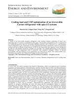
Figure 2 shows the finite time exergoeconomic performance characteristics of the irreversible universal
heat pump cycle with variable-temperature heat reservoirs. Heat conductances of the hot- and cold-side
heat exchangers are set as U H 1 = 0 , U L 2 = 0 and U H 2 = U L1 = 3 kW / K for Brayton, Otto, Diesel and
Atkinson heat pump cycles; U H 1 = U H 2 = U L1 = 2 kW / K and U L 2 = 0 for Dual heat pump cycle; U H 1 = 0
and U H 2 = U L1 = U L 2 = 2 kW / K for Miller heat pump cycle, respectively. Internal irreversibility and price
ratio are set as φ = 1.1 and ψ 1 ψ 2 = 5 , respectively. One can continue to discuss the special cases of the
universal heat pump cycle for different thermal capacity rates of the working fluid ( Cwf 1 , Cwf 2 , Cwf 3 and
Cwf 4 ) in detail, whose dimensionless profit rate versus COP curves are also shown in Figure 2.

Figure 2. Π vs. β characteristics of irreversible universal heat pump cycle with variable-temperature
heat reservoirs
&
&
(1) When Cwf 1 = Cwf 2 = mC p (mass flow rate m of the working fluid and constant pressure specific heat
&
C p product) and Cwf 3 = Cwf 4 = mC p , U H 1 = 0 , U L 2 = 0 and x = y = 1 , equations (30) and (33) become the
COP and finite time exergoeconomic performance characteristics of an irreversible variable-temperature
heat reservoir steady flow Brayton heat pump cycle with the losses of heat-resistance and internal
irreversibility.

ISSN 2076-2895 (Print), ISSN 2076-2909 (Online) ©2010 International Energy & Environment Foundation. All rights reserved.


976

International Journal of Energy and Environment (IJEE), Volume 1, Issue 6, 2010, pp.969-986

&
&
(2) When Cwf 1 = Cwf 2 = mCv (mass flow rate m of the working fluid and constant volume specific heat Cv
&
product) and Cwf 3 = Cwf 4 = mCv , U H 1 = 0 , U L 2 = 0 and x = y = 1 , equations (30) and (33) become the COP
and finite time exergoeconomic performance of an irreversible variable-temperature heat reservoir steady
flow Otto heat pump cycle with the losses of heat-resistance and internal irreversibility.
&
&
(3) When Cwf 1 = Cwf 2 = mCv and Cwf 3 = Cwf 4 = mC p , U H 1 = 0 , U L 2 = 0 and x = y = 1 , equations (30) and
(33) become the COP and finite time exergoeconomic performance characteristics of an irreversible

variable-temperature heat reservoir steady flow Diesel heat pump cycle with the losses of heat-resistance
and internal irreversibility.
&
&
(4) When Cwf 1 = Cwf 2 = mC p and Cwf 3 = Cwf 4 = mCv , U H 1 = 0 , U L 2 = 0 and x = y = 1 , equations (30) and
(33) become the COP and finite time exergoeconomic performance characteristics of an irreversible
variable-temperature heat reservoir steady flow Atkinson heat pump cycle with the losses of heatresistance and internal irreversibility.
&
&
&
(5) When Cwf 1 = Cwf 2 = mCv , Cwf 3 = mCv and Cwf 4 = mC p , U H 1 ≠ 0 , U H 2 ≠ 0 , U L 2 = 0 and y = 1 , equations
(30) and (33) become the COP and finite time exergoeconomic performance characteristics of an
irreversible variable-temperature heat reservoir steady flow Dual heat pump cycle with the losses of heatresistance and internal irreversibility. If U H 1 → 0 , U L 2 = 0 and x = y = 1 further, the Dual heat pump
cycle is close to the Diesel heat pump cycle. If U H 2 → 0 , U L 2 = 0 and y = 1 further, the Dual heat pump
cycle is close to the Otto heat pump cycle.
In this case, the range of x becomes:

1 ≤ x ≤ [CH 1min CH 2 min Cwf 3 E H 1E H 2 (−T6 + THin ) / CH + CH 1min E H 1THin (−Cwf 4 + CH 2 min E H 2 ) +
Cwf 3 (Cwf 4T6 − CH 2 min E H 2THin )] [T6 (Cwf 3 − CH 1min E H 1 )(Cwf 4 − CH 2 min E H 2 )]

(38)

and the value of x is given by:
x = T5 / T6 = [CH 1min CH 2 min Cwf 3 E H 1E H 2 ( −T6 + THin ) / CH + CH 1min E H 1THin (−Cwf 4 + CH 2 min E H 2 ) +
Cwf 3 (Cwf 4T6 − CH 2 min E H 2THin )] [(Cwf 3T6 − CH 1min EH 1THin )(Cwf 2 − CH 2 min E H 2 )]

(39)

&
&

&
(6) When Cwf 1 = mC p , Cwf 2 = mCv and Cwf 3 = Cwf 4 = mCv , U H 1 = 0 , U L1 ≠ 0 , U L 2 ≠ 0 and x = 1 , equations
(30) and (33) become the COP and finite time exergoeconomic performance characteristics of an
irreversible variable-temperature heat reservoir steady flow Miller heat pump cycle with the losses of
heat-resistance and internal irreversibility. If U H 1 = 0 , U L 2 → 0 and x = y = 1 further, the Miller heat
pump cycle is close to the Atkinson heat pump cycle. If U H 1 = 0 , U L1 → 0 and x = 1 further, the Miller
heat pump cycle is close to the Otto heat pump cycle.
In this case, the range of y is:
1

⎧[CH 1min CH 2 min Cwf 3 E H 1E H 2 ( −T6 + THin ) / CH + CH 1min E H 1THin (−Cwf 4 + CH 2 min E H 2 ) + ⎫φ
⎪
⎪
1≤ y ≤ ⎨
⎬
Cwf 3 (Cwf 4T6 − CH 2 min E H 2THin )] [(Cwf 3T6 − CH 1 min EH 1THin )(Cwf 2 − CH 2 min E H 2 )] ⎪
⎪
⎩
⎭

(40)

Combining equations (18), (19) and (22) give the following equation that the working fluid temperature
T3 should satisfy:
1

(Cwf 1 − CL1min E L1 )(Cwf 2T3 − CL 2 min EL 2TLin )[T3 (Cwf 2 − CL 2 min EL 2 ) / (Cwf 2T3 − CL 2 min EL 2TLin )]k /
[CL1min CL 2 min Cwf 2 E L1E L 2 (TLin − T3 ) CL + CL1min E L1TLin (CL 2 min E L 2 − Cwf 2 ) + Cwf 1 (Cwf 2T3 − CL 2 min E L 2TLin )] =
⎧[CH 1min CH 2 min Cwf 3 E H 1E H 2 (−T6 + THin ) / CH + CH 1min E H 1THin (−Cwf 4 + CH 2 min E H 2 ) + ⎫
⎪

⎪
⎨
⎬
⎪ Cwf 3 (Cwf 4T6 − CH 2 min E H 2THin )] [(Cwf 3T6 − CH 1min EH 1THin )(Cwf 2 − CH 2 min E H 2 )] ⎪
⎩
⎭

(41)

1
φk

ISSN 2076-2895 (Print), ISSN 2076-2909 (Online) ©2010 International Energy & Environment Foundation. All rights reserved.


International Journal of Energy and Environment (IJEE), Volume 1, Issue 6, 2010, pp.969-986

977

where k is the ratio of the specific heats. Moreover, combining equations (18), (19), (21) with equation
(41) gives G and y .
(7) When Cwf 1 = Cwf 2 = Cwf 3 = Cwf 4 → ∞ , equations (30) and (33) become the COP and finite time
exergoeconomic performance characteristics of an irreversible variable-temperature heat reservoir steady
flow Carnot heat pump cycle with the losses of heat-resistance and internal irreversibility. Specially, if
CH → ∞ and CL → ∞ further, the finite time exergoeconomic performance characteristic of an
irreversible Carnot heat pump cycle with variable-temperature heat reservoirs become the finite time
exergoeconomic performance characteristics of endoreversible ( φ = 1 ) [21, 24] and irreversible ( φ > 1 )
[28] Carnot heat pump cycle with constant-temperature heat reservoirs, respectively.
5. Finite time exergoeconomic performance optimization
5.1 Optimal distributions of heat conductance

If heat conductances of hot- and cold-side heat exchangers are changeable, the profit rate of the
irreversible universal heat pump cycle may be optimized by searching the optimal heat conductance
distributions for the fixed total heat exchanger inventory. For the fixed heat exchanger inventory U T , that
is, for the constraint of U H 1 + U H 2 + U L1 + U L 2 = U T , defining the distributions of heat conductance
uH 1 = U H 1 / U T , uH 2 = U H 2 / U T , uL1 = U L1 / U T and uL 2 = U L 2 / U T leads to:

U H 1 = u H 1U T , U H 2 = u H 2U T , U L1 = u L1U T , U L1 = u L1U T , U L 2 = u L 2U T

(42)

The following conditions should be satisfied: 0 ≤ uH 1 ≤ 1 , 0 ≤ uH 2 ≤ 1 , 0 ≤ uL1 ≤ 1 , 0 ≤ uL 2 ≤ 1 , and
u H 1 + u H 2 + u L1 + u L 2 = 1 . Moreover, heat conductance distributions are set as uH 1 = 0 and uL 2 = 0 for
Brayton, Otto, Diesel and Atkinson heat pump cycles; uL 2 = 0 for Dual heat pump cycle; uH 1 = 0 for
Miller heat pump cycle, respectively.
To illustrate the preceding analyses, one can take the irreversible Brayton heat pump cycle with variabletemperature heat reservoirs (air as the working fluid) as a numerical example. In the calculations, it is set
that THin = 290.0K , TLin = 268.0K , CH = CL = 1.2 kW / K , Cv = 0.7165kJ / (kg ⋅ K ) , C p = 1.0031kJ / (kg ⋅ K ) ,
&
k = 1.4 , φ = 1.1 , U T = 5 kW / K , m = 1.1165kg / s and ψ 1 / ψ 2 = 5 . If there are no special explanations, the
parameters are set as above. The working fluid temperature T6 is a variable and its reasonable value is
greater than THin . The calculations illustrate that the values of x and y are always in their ranges. The
&
dimensionless profit rate is defined as Π = Π (0.9mTL CVψ 2 ) .

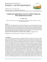
Figure 3 shows the effect of the price ratio (ψ 1 ψ 2 ) on the dimensionless profit rate ( Π ) versus COP
( β ) for irreversible variable-temperature heat reservoir Brayton heat pump cycle. From Figure 3, one
can see that Π increases with the increase in ψ 1 ψ 2 for the fixed β . Moreover, when ψ 1 ψ 2 = 1 , the
maximum profit rate is not greater than zero, i.e., the heat pump is not profitable regardless of any
working condition.
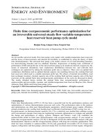
The dimensionless profit rate ( Π ) versus COP ( β ) and the hot-side heat conductance distribution ( uH 2 )
of an irreversible variable-temperature heat reservoir Brayton heat pump cycle with ψ 1 ψ 2 = 5 and

φ = 1.1 is shown in Figure 4. It indicates that the curve of dimensionless profit rate versus hot-side heat
conductance distribution is a parabolic-like one for the fixed COP. There exists an optimal heat
conductance distribution ( uH 2,opt ,Π ) which leads to the optimal dimensionless profit rate ( Π opt , u ). For Otto,
Diesel and Atkinson heat pump cycles, the three-dimensional diagram characteristics among
dimensionless profit rate versus COP and heat conductance distribution are similar with those shown in
Figure 4.
The three-dimensional diagram among the dimensionless profit rate ( Π ) and heat conductance
distributions ( uH 1 and uH 2 ) of an irreversible variable-temperature heat reservoir Dual heat pump cycle
with β = 3 , ψ 1 ψ 2 = 5 and φ = 1.1 is shown in Figure 5. It indicates that there exists a pair of uH 1,opt , Π near
zero and uH 2, opt ,Π near 0.5 , which lead to the optimal dimensionless profit rate. In this case, Dual heat
pump cycle becomes Diesel heat pump cycle. The three-dimensional diagram among the dimensionless
ISSN 2076-2895 (Print), ISSN 2076-2909 (Online) ©2010 International Energy & Environment Foundation. All rights reserved.


978

International Journal of Energy and Environment (IJEE), Volume 1, Issue 6, 2010, pp.969-986

profit rate ( Π ) and heat conductance distributions ( uL1 and uL 2 ) of an irreversible variable-temperature
heat reservoir Miller heat pump cycle with β = 3 , ψ 1 ψ 2 = 5 and φ = 1.1 is shown in Figure 6. It indicates
that there exists a pair of u L1, opt , Π near 0.5 and u L 2, opt , Π near zero, which lead to the optimal
dimensionless profit rate. In this case, Miller heat pump cycle becomes Atkinson heat pump cycle.
Figure 7 show the optimal heat conductance distribution ( uH 2,opt ,Π ) versus COP ( β ) for Brayton, Otto,
Diesel and Atkinson heat pump cycles. It indicates that u H 2, opt , Π is a little greater than 0.5 for Brayton,
Otto, Diesel and Atkinson heat pump cycles, and the COP has little effects on u H 2, opt , Π . Moreover, when
carrying out heat conductance optimizations, u H 2, opt , Π for Dual heat pump cycle and uL 2,opt ,Π for Miller
heat pump cycle are close to the corresponding optimal heat conductance distributions of Diesel and
Atkinson heat pump cycles as shown in Figures 5 and 6, respectively.

Figure 3. Effect of ψ 1 / ψ 2 on Π vs. β characteristic for irreversible variable-temperature heat reservoir

Brayton heat pump cycle

Figure 4. Π vs. β and uH 2 for irreversible variable-temperature heat reservoir Brayton heat pump cycle

ISSN 2076-2895 (Print), ISSN 2076-2909 (Online) ©2010 International Energy & Environment Foundation. All rights reserved.


International Journal of Energy and Environment (IJEE), Volume 1, Issue 6, 2010, pp.969-986

979

Figure 5. Π vs. uH 1 and uH 2 for irreversible variable-temperature heat reservoir Dual heat pump cycle

Figure 6. Π vs. uL1 and uL 2 for irreversible variable-temperature heat reservoir Miller heat pump cycle

Figure 7. u H 2 opt , Π vs. β for irreversible variable-temperature heat reservoir Brayton, Otto, Diesel and
Atkinson heat pump cycles
ISSN 2076-2895 (Print), ISSN 2076-2909 (Online) ©2010 International Energy & Environment Foundation. All rights reserved.


980

International Journal of Energy and Environment (IJEE), Volume 1, Issue 6, 2010, pp.969-986

5.2 Optimal finite time exergoeconomic performance
Figure 8 shows the optimal dimensionless profit rate ( Π opt , u ) versus COP ( β ) characteristic for
irreversible variable-temperature heat reservoir Brayton, Otto, Diesel, Atkinson, Dual and Miller heat
pump cycles with ψ 1 ψ 2 = 5 and φ = 1.1 . It indicates that Π opt , u decreases with the increase in β . Dual
and Diesel, Miller and Atkinson heat pump cycles have the same optimal dimensionless profit rate versus
COP characteristics, respectively. For the fixed β , Brayton heat pump cycle has the maximum Π opt , u

among the six heat pump cycles, and Otto heat pump cycle has the minimum.

Figure 8. Π opt , u vs. β characteristics for six heat pump cycles
Figures 9-11 show the effect of internal irreversibility ( φ ), total heat exchanger inventory ( U T ) and
thermal capacity rate of the working fluid ( Cwf 4 ) on the optimal dimensionless profit rate ( Π opt ,u ) versus
COP ( β ) characteristics of an irreversible variable-temperature heat reservoir Brayton heat pump cycle
with ψ 1 ψ 2 = 5 and CH = CL = 1.2 kW / K , respectively. From Figure 9, one can see that for the fixed
COP, Π opt ,u decreases with the increase in φ . Moreover, when φ = 1 , Π opt ,u versus β characteristic of an
irreversible Brayton heat pump cycle with variable-temperature heat reservoirs becomes that of an
endoreversible one. From Figure 10, one can see that Π opt ,u increases with the increase of U T for the
fixed β , but the increment decreases gradually. From Figure 11, one can see that Π opt ,u increases with
the increase of Cwf 4 when Cwf 4 is lower than CH and CL ; Π opt ,u decreases with the increase of Cwf 4
when Cwf 4 is greater than CH and CL . Moreover, the effects of internal irreversibility, total heat
exchanger inventory and thermal capacity rate of the working fluid on the optimal finite time
exergoeconomic performances of Otto, Diesel, Atkinson, Dual and Miller heat pump cycles are similar
with those shown in Figures 9-11.

ISSN 2076-2895 (Print), ISSN 2076-2909 (Online) ©2010 International Energy & Environment Foundation. All rights reserved.


International Journal of Energy and Environment (IJEE), Volume 1, Issue 6, 2010, pp.969-986

981

Figure 9. Effect of φ on Π opt , u vs. β characteristic for irreversible variable-temperature heat reservoir
Brayton heat pump cycle

Figure 10. Effect of U T on Π opt , u vs. β characteristic for irreversible variable-temperature heat reservoir
Brayton heat pump cycle

Figure 11. Effect of Cwf 4 on Π opt , u vs. β characteristic for irreversible variable-temperature heat
reservoir Brayton heat pump cycle
ISSN 2076-2895 (Print), ISSN 2076-2909 (Online) ©2010 International Energy & Environment Foundation. All rights reserved.


982

International Journal of Energy and Environment (IJEE), Volume 1, Issue 6, 2010, pp.969-986

5.3 Optimal thermal capacity rate matching between the working fluid and heat reservoirs
Figure 12 shows a three-dimensional diagram among the dimensionless profit rate ( Π ), thermal capacity
rate matching ( c = Cwf 4 / CL ) between the working fluid and heat reservoirs and heat conductance
distribution ( uH 2 ) of an irreversible variable-temperature heat reservoir Brayton heat pump cycle with
β = 3 , ψ 1 ψ 2 = 5 and φ = 1.1 . From Figure 12, one can see that the curve of Π versus c is a paraboliclike one for the fixed uH 2 . There exist an optimal thermal capacity rate matching ( copt ) between the

working fluid and heat reservoirs and an optimal heat conductance distribution ( uH 2, opt ) which lead to the
double maximum dimensionless profit rate.
Figures 13-15 show the effect of internal irreversibility ( φ ), total heat exchanger inventory ( U T ) and
heat capacity ratio of the heat reservoirs ( CH / CL ) on the optimal dimensionless profit rate ( Π opt ,u ) versus
thermal capacity rate matching ( c ) between the working fluid and heat reservoirs characteristics of an
irreversible variable-temperature heat reservoir Brayton heat pump cycle with ψ 1 ψ 2 = 5 , respectively.
From Figure 13, for the fixed c , Π opt ,u decreases with the increase in φ . Moreover, when φ = 1 , Π opt ,u
versus c characteristic of an irreversible Brayton heat pump cycle with variable-temperature heat
reservoirs becomes that of an endoreversible one. From Figure 14, one can see that Π opt ,u increases with
the increase in U T for the fixed c , but the increment decreases gradually. From Figure 15, one can see
that when CH / CL = 1 , the optimal thermal capacity rate matching between the working fluid and heat
reservoirs is copt = 1 , which leads to the double maximum dimensionless profit rate. Meanwhile, copt
increases with the increase in CH / CL . Moreover, the effects of internal irreversibility, total heat
exchanger inventory and heat capacity ratio of the heat reservoirs on the optimal finite time
exergoeconomic performances of Otto, Diesel, Atkinson, Dual and Miller heat pump cycles are similar

with those shown in Figures 13-15.

Figure 12. Π vs. c and uH 2 for irreversible variable-temperature heat reservoir Brayton heat pump cycle

ISSN 2076-2895 (Print), ISSN 2076-2909 (Online) ©2010 International Energy & Environment Foundation. All rights reserved.


International Journal of Energy and Environment (IJEE), Volume 1, Issue 6, 2010, pp.969-986

983

Figure 13. Effect of φ on Π opt , u vs. c characteristic for irreversible variable-temperature heat reservoir
Brayton heat pump cycle

Figure 14. Effect of U T on Π opt , u vs. c characteristic for irreversible variable-temperature heat reservoir
Brayton heat pump cycle

Figure 15. Effect of CH / CL on Π opt , u vs. c characteristic for irreversible variable-temperature heat
reservoir Brayton heat pump cycle
ISSN 2076-2895 (Print), ISSN 2076-2909 (Online) ©2010 International Energy & Environment Foundation. All rights reserved.


984

International Journal of Energy and Environment (IJEE), Volume 1, Issue 6, 2010, pp.969-986

6. Conclusion
Finite time exergoeconomic performance of an irreversible universal steady flow heat pump cycle model
with variable-temperature heat reservoirs, and the losses of heat transfer and internal irreversibility is
analyzed and optimized by using the theory of finite time thermodynamics. Expressions for COP and

profit rate are derived and are used to discuss the optimal finite time exergoeconomic performance of the
universal heat pump cycle. Numerical examples show that the optimal hot-side heat conductance
distributions are a little greater than 0.5 for Brayton, Otto, Diesel and Atkinson heat pump cycles;
optimal performances of Dual and Miller heat pump cycles are close to those of Diesel and Atkinson heat
pump cycles, respectively. There exist an optimal heat conductance distribution and an optimal thermal
capacity rate matching between the working fluid and heat reservoirs which lead to the double maximum
profit rate. Moreover, the effects of internal irreversibility, total heat exchanger inventory, thermal
capacity rate of the working fluid and heat capacity ratio of the heat reservoirs on the optimal finite time
exergoeconomic performance and optimal thermal capacity rate matching between the working fluid and
heat reservoirs are discussed. The results obtained herein include the optimal finite time exergoeconomic
performance of endoreversible and irreversible, constant- and variable- temperature heat reservoir
Brayton, Otto, Diesel, Atkinson, Dual, Miller and Carnot heat pump cycles, and can provide some
theoretical guidelines for parameter designs and performance optimizations of various practical heat
pumps.
Acknowledgements
This paper is supported by The National Natural Science Foundation of P. R. China (Project No.
10905093), The Program for New Century Excellent Talents in University of P. R. China (Project No.
NCET-04-1006) and The Foundation for the Author of National Excellent Doctoral Dissertation of P. R.
China (Project No. 200136).
References
[1] Novikov II. The efficiency of atomic power stations (A review). Atommaya Energiya 3, 1957(11):
409.
[2] Chambdal P. Les Centrales Nucleases. Paris: Armand Colin, 1957(11): 41-58.
[3] Curzon F L, Ahlborn B. Efficiency of a Carnot engine at maximum power output. Am. J. Phys.,
1975, 43(1): 22-24.
[4] Andresen B. Finite-Time Thermodynamics. Physics Laboratory , University of Copenhagen,
1983.
[5] Andresen B, Salamon P and Berry R S. Thermodynamics in finite time. Phys. Today, 1984 (Sept.):
62-70.
[6] Andresen B, Berry R S, Ondrechen M J, Salamon P. Thermodynamics for processes in finite time.

Acc. Chem. Res. 1984, 17(8): 266-271.
[7] Sieniutycz S, Shiner J S. Thermodynamics of irreversible processes and its relation to chemical
engineering: Second law analyses and finite time thermodynamics. J. Non-Equilib. Thermodyn.,
1994, 19(4): 303-348.
[8] Bejan A. Entropy generation minimization: The new thermodynamics of finite-size device and
finite-time processes. J. Appl. Phys., 1996, 79(3): 1191-1218.
[9] Feidt M. Thermodynamique et Optimisation Energetique des Systems et Procedes (2nd Ed.). Paris:
Technique et Documentation, Lavoisier, 1996.
[10] Hoffmann K H, Burzler J M and Schubert S. Endoreversible Thermodynamics. J. Non-Equilib.
Thermodyn., 1997, 22(4): 311-355.
[11] Berry R S, Kazakov V A, Sieniutycz S, Szwast Z, Tsirlin A M. Thermodynamic Optimization of
Finite Time Processes. Chichester: Wiley, 1999.
[12] Chen L, Wu C, Sun F. Finite time thermodynamic optimization or entropy generation
minimization of energy systems. J. Non-Equilib. Thermodyn., 1999, 24(4): 327-359.
[13] Sieniutycz S. Thermodynamic limits on production or consumption of mechanical energy in
practical and industry systems. Progress Energy & Combustion Sci., 2003, 29(3): 193-246.
[14] Feidt M. Optimal use of energy systems and processes. Int. J. Exergy, 2008, 5(5/6): 500-531.
[15] Sieniutycz S, Jezowski J. Energy Optimization in Process Systems. Oxford: Elsevier, 2009.
[16] Tsatsaronts G. Thermoeconomic analysis and optimization of energy systems. Progress Energy &
Combustion Sci., 1993, 19(3): 227-257.
ISSN 2076-2895 (Print), ISSN 2076-2909 (Online) ©2010 International Energy & Environment Foundation. All rights reserved.


International Journal of Energy and Environment (IJEE), Volume 1, Issue 6, 2010, pp.969-986

985

[17] El-Sayed M Y. The Thermoeconomics of Energy Conversion. London: Elsevier, 2003.
[18] Salamon P, Nitzan A. Finite time optimizations of a Newton's law Carnot cycle. J. Chem. Phys.,
1981, 74(6): 3546-3560.

[19] Chen L, Sun F and Chen W. Finite time exergoeconomic performance bound and optimization
criteria for two-heat-reservoir refrigerators. Chinese Sci. Bull., 1991, 36(2): 156-157 (in Chinese).
[20] Chen L, Sun F, Wu C. Exergoeconomic performance bound and optimization criteria for heat
engines. Int. J. Ambient Energy, 1997, 18(4): 216-218.
[21] Chen L, Sun F. The maximum profit rate characteristic of Carnot heat pump. Practice Energy
Source, 1993(3): 29-30 (in Chinese).
[22] Wu C, Chen L, Sun F. Effect of heat transfer law on finite time exergoeconomic performance of
heat engines. Energy, The Int. J., 1996, 21(12): 1127-1134.
[23] Chen L, Wu C, Sun F. Effect of heat transfer law on finite time exergoeconomic performance of a
Carnot refrigerator. Exergy, An Int. J., 2001, 1(4): 295-302.
[24] Wu C, Chen L, Sun F. Effect of heat transfer law on finite time exergoeconomic performance of a
Carnot heat pump. Energy Convers. Mgmt., 1998, 39(7): 579-588.
[25] Chen L, Sun F, Wu C. Maximum profit performance for generalized irreversible Carnot engines.
Appl. Energy, 2004, 79(1): 15-25.
[26] Chen L, Zheng Z, Sun F, Wu C. Profit performance optimization for an irreversible Carnot
refrigeration cycle. Int. J. Ambient Energy, 2008, 29(4): 197-206.
[27] Chen L, Zheng Z, Sun F. Maximum profit performance for a generalized irreversible Carnot heat
pump cycle. Termotehnica, 2008, 12(2): 22-26.
[28] Zheng Z, Chen L, Sun F, Wu C. Maximum profit performance for a class of universal steady flow
endoreversible heat engine cycles. Int. J. Ambient Energy, 2006, 27(1): 29-36.
[29] Kan X, Chen L, Sun F, Wu F. Exergoeconomic performance optimization for a steady flow
endoreversible refrigerator cycle model including five typical cycles. Int. J. Low-Carbon Tech.,
2010, 5(2), 74-80.
[30] Feng H, Chen L, Sun F. Finite time exergoeconomic performance optimization for a universal
steady flow endoreversible heat pump model. Int. J. Low-Carbon Tech., 2010, 5(2), 105-110.
[31] Feng H, Chen L, Sun F. Finite time exergoeconomic performance optimization for a universal
steady flow irreversible heat pump model. Int. J. Sustainable Energy, 2010, in press.
[32] Chen L, Sun F, Wu C. Maximum profit performance of an absorption refrigerator. Int. J. Energy,
Environment, and Economics, 1996, 4(1): 1-7.
[33] Chen L, Wu C, Sun F, Cao S. Maximum profit performance of a three-heat-reservoir heat pump.

Int. J. Energy Res., 1999, 23(9): 773-777.
[34] Qin X, Chen L, Sun F, Wu C. Thermoeconomic optimization of an endoreversible four-heatreservoir absorption-refrigerator. Appl. Energy, 2005, 81(4): 420-433.
[35] Tao G, Chen L, Sun F. Exergoeconomic performance optimization for an endoreversible simple
gas turbine closed-cycle cogeneration plant. Int. J. Ambient Energy, 2009, 30(3): 115-124.
[36] Tao G, Chen L, Sun F. Exergoeconomic performance optimization for an endoreversible
regenerative gas turbine closed-cycle cogeneration plant. Rev. Mex. Fis., 2009, 55(3): 192-200.
[37] Sahin B, Kodal A. Performance analysis of an endoreversible heat engine based on a new
thermoeconomic optimization criterion. Energy Convers. Mgmt., 2001, 42(9): 1085-1093.
[38] Sahin B, Kodal A. Finite time thermoeconomic optimization for endoreversible refrigerators and
heat pumps. Energy Convers. Mgmt., 1999, 40(9): 951-960.
[39] Kodal A, Sahin B. Finite time thermoeconomic optimization for irreversible heat engines. Int. J.
Thermal Sci., 2003, 42(8): 777-782.
[40] Kodal A, Sahin B, Yilmaz T. Effects of internal irreversibility and heat leakage on the finite time
thermoeconomic performance of refrigerators and heat pumps. Energy Convers. Mgmt., 2000,
41(6): 607-619.
[41] Kodal A, Sahin B, Ekmekci I, Yilmaz T. Thermoeconomic optimization for irreversible absorption
refrigerators and heat pumps. Energy Convers. Mgmt., 2003, 44(1): 109-123.
[42] Chen L, Shen L, Sun F. Performance comparison for endoreversible Carnot and Brayton heat
pumps. II. Steady flow cycles with finite reservoirs. Power System Engng., 1996, 12(5): 1-5 (in
Chinese).
[43] Wu C, Chen L, Sun F. Optimization of steady flow heat pumps. Energy Convers. Mgnt., 1998,
39(5/6): 445-453.
ISSN 2076-2895 (Print), ISSN 2076-2909 (Online) ©2010 International Energy & Environment Foundation. All rights reserved.


986

International Journal of Energy and Environment (IJEE), Volume 1, Issue 6, 2010, pp.969-986

[44] Bi Y, Chen L, Sun F. Heating load, heating load density and COP optimizations for an

endoreversible variable-temperature heat reservoir air heat pump. J. Energy Institute, 2009, 82(1):
43-47.
[45] Bi Y, Chen L, Sun F. Ecological, exergetic efficiency and heating load optimizations for
irreversible variable-temperature heat reservoir simple air heat pump cycles. Ind. J. Pure Appl.
Phys., 2009, 47(12): 852-862.

Huijun Feng received his BS Degree from the Naval University of Engineering, P R China in 2008. He is
pursuing for his MS Degree in power engineering and engineering thermophysics from Naval University
of Engineering, P R China. His work covers topics in finite time thermodynamics and technology support
for propulsion plants. He has published ten papers in the international journals.

Lingen Chen received all his degrees (BS, 1983; MS, 1986, PhD, 1998) in power engineering and
engineering thermophysics from the Naval University of Engineering, P R China. His work covers a
diversity of topics in engineering thermodynamics, constructal theory, turbomachinery, reliability
engineering, and technology support for propulsion plants. He has been the Director of the Department of
Nuclear Energy Science and Engineering and the Director of the Department of Power Engineering. Now,
he is the Superintendent of the Postgraduate School, Naval University of Engineering, P R China.
Professor Chen is the author or coauthor of over 1050 peer-refereed articles (over 460 in English journals)
and nine books (two in English).
E-mail address: ; , Fax: 0086-27-83638709 Tel: 0086-2783615046

Fengrui Sun received his BS Degrees in 1958 in Power Engineering from the Harbing University of
Technology, P R China. His work covers a diversity of topics in engineering thermodynamics, constructal
theory, reliability engineering, and marine nuclear reactor engineering. He is a Professor in the Department
of Power Engineering, Naval University of Engineering, P R China. Professor Sun is the author or coauthor of over 750 peer-refereed papers (over 340 in English) and two books (one in English).

ISSN 2076-2895 (Print), ISSN 2076-2909 (Online) ©2010 International Energy & Environment Foundation. All rights reserved.