Exergoeconomic performance optimization for a steadyflow endoreversible refrigeration model including six typical cycles

I
NTERNATIONAL
J
OURNAL OF

E
NERGY AND
E
NVIRONMENT



Volume 4, Issue 1, 2013 pp.93-102

Journal homepage: www.IJEE.IEEFoundation.org


ISSN 2076-2895 (Print), ISSN 2076-2909 (Online) ©2013 International Energy & Environment Foundation. All rights reserved.
Exergoeconomic performance optimization for a steady-
flow endoreversible refrigeration model including six typical
cycles


Lingen Chen, Xuxian Kan, Fengrui Sun, Feng Wu

College of Naval Architecture and Power, Naval University of Engineering, Wuhan 430033, P. R. China.


Abstract
The operation of a universal steady flow endoreversible refrigeration cycle model consisting of a
constant thermal-capacity heating branch, two constant thermal-capacity cooling branches and two

adiabatic branches is viewed as a production process with exergy as its output. The finite time
exergoeconomic performance optimization of the refrigeration cycle is investigated by taking profit rate
optimization criterion as the objective. The relations between the profit rate and the temperature ratio of
working fluid, between the COP (coefficient of performance) and the temperature ratio of working fluid,
as well as the optimal relation between profit rate and the COP of the cycle are derived. The focus of this
paper is to search the compromised optimization between economics (profit rate) and the utilization
factor (COP) for endoreversible refrigeration cycles, by searching the optimum COP at maximum profit,
which is termed as the finite-time exergoeconomic performance bound. Moreover, performance analysis
and optimization of the model are carried out in order to investigate the effect of cycle process on the
performance of the cycles using numerical example. The results obtained herein include the performance
characteristics of endoreversible Carnot, Diesel, Otto, Atkinson, Dual and Brayton refrigeration cycles.
Copyright © 2013 International Energy and Environment Foundation - All rights reserved.

Keywords: Finite-time thermodynamics; Endoreversible refrigeration cycle; Exergoeconomic
performance



1. Introduction
Recently, the analysis and optimization of thermodynamic cycles for different optimization objectives
has made tremendous progress by using finite-time thermodynamic theory [1-14]. Finite-time
thermodynamics is a powerful tool for the performance analysis and optimization of various cycles. For
refrigeration cycles, the performance analysis and optimization have been carried out by taking cooling
load, coefficient of performance (COP), specific cooling load, cooling load density, exergy destruction,
exergy output, exergy efficiency, and ecological criteria as the optimization objectives in much work,
and many meaningful results have been obtained [15-27].
A relatively new method that combines exergy with conventional concepts from long-run engineering
economic optimization to evaluate and optimize the design and performance of energy systems is
exergoeconomic (or thermoeconomic) analysis [28, 29]. Salamon and Nitzan’s work [30] combined the
endoreversible model with exergoeconomic analysis. It was termed as finite time exergoeconomic

analysis [31-45] to distinguish it from the endoreversible analysis with pure thermodynamic objectives
and the exergoeconomic analysis with long-run economic optimization. Similarly, the performance
International Journal of Energy and Environment (IJEE), Volume 4, Issue 1, 2013, pp.93-102
ISSN 2076-2895 (Print), ISSN 2076-2909 (Online) ©2013 International Energy & Environment Foundation. All rights reserved.

94
bound at maximum profit was termed as finite time exergoeconomic performance bound to distinguish it
from the finite time thermodynamic performance bound at maximum thermodynamic output.
There have been some papers concerning finite time exergoeconomic optimization for refrigeration
cycles [31, 33, 38]. A further step in this paper is to build a universal endoreversible steady flow
refrigeration cycle model consisting of a constant thermal-capacity heating branch, two constant thermal-
capacity cooling branches and two adiabatic branches with the consideration of heat resistance loss. The
finite time exergoeconomic performance of the universal endoreversible refrigeration cycles is studied.
The relations between the profit rate and the temperature ratio of working fluid, between the COP and the
temperature ratio of working fluid, as well as the optimal relation between profit rate and the COP of the
cycle are derived. The focus of this paper is to search the compromise optimization between economics
(profit rate) and the energy utilization factor (COP) for the endoreversible refrigeration cycles. Moreover,
performance analysis and optimization of the model are carried out in order to investigate the effect of
cycle process on the performance of the cycles using numerical examples. The results obtained herein
include the performance characteristics of endoreversible Carnot, Diesel, Otto, Atkinson, Dual and
Brayton refrigeration cycles.

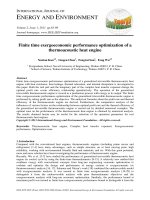
2. Cycle model
An endoreversible steady flow referigeration cycle operating between an infinite heat sink at temperature
H
T
and an infinite heat source at temperature
L
T
is shown in Figure 1. In this T-s diagram, the processes

between 2 and 3 , as well as between 5 and 1 are two adiabatic branches; the process between 1 and 2 is a
heating branch with constant thermal capacity (mass flow rate and specific heat product)
in
C
; the
processes between 3 and 4, and 4 and 5 are two cooling branches with constant thermal capacity
1
out
C
and
2
out
C
. In addition, the heat conductances (heat transfer coefficient-area product) of the hot- and cold-side
heat exchangers are
1
H
U
,
2
H
U
, and
L
U
, respectively. The heat exchanger inventory is taken as a constant,
that is
12
H HLT
UUUU++=

. This cycle model is more generalized. If
in
C
,
1
out
C
and
2
out
C
have different values,
the model can become various special endoreversible refrigeration cycle models.



Figure 1. T-s diagram for universal endoreversible cycle model

3. Performance analysis
According to the properties of working fluid and the theory of heat exchangers, the rate of heat transfer
1H
Q
and
2H
Q
released to the heat sink and the rate of heat transfer
L
Q
(i. e. the cooling load
R

) supplied by
heat source are given, respectively, by

12H HH
QQQ
=+
(1)

..
1134 113
() ( )
H out out H H
QmCTTmCETT=−= −
(2)

..
2245 224
() ( )
H out out H H
QmCTTmCETT=−= −
(3)

..
21 1
() ()
Lin inLL
R QmCTTmCETT== −= −
(4)

International Journal of Energy and Environment (IJEE), Volume 4, Issue 1, 2013, pp.93-102

ISSN 2076-2895 (Print), ISSN 2076-2909 (Online) ©2013 International Energy & Environment Foundation. All rights reserved.

95
where
m

is mass flow rate of the working fluid,
1H
E
,
2H
E
and
L
E
are the effectivenesses of the hot- and
cold-side heat exchangers, and are defined as

11
1exp( )
HH
EN=− −
,
22
1 exp( )
HH
EN=− −
,
1exp( )
L L

EN=− −
(5)

where
1H
N
,
2H
N
and
L
N
are the numbers of heat transfer units of the hot- and cold-side heat exchangers,
and are defined as

.
11 1
/( )
H Hout
NUmC=
,
.
22 2
/( )
H H out
NUmC=
,
.
/( )
L Lin

NUmC=
(6)

where
1H
U
,
2H
U
and
L
U
are the heat conductance, that is, the product of heat transfer coefficient
α
and
heat transfer surface area
F


111H HH
UF
α
=
,
222H HH
UF
α
=
,
L LL

UF
α
=
(7)

The COP
ε
of the cycle is

()()
1
1
12
11
HL H H L
QQ Q Q Q
ε
−
−
=−=+ −
⎡⎤
⎣⎦
(8)

Combining equations (1) - (3) and (8) gives

41 1
(1 )
H HHL
TET ExT=+−

(9)

()
512 1212
(1 )(1 )
H HL HH HHH
TEExTEEEET=− − + + −
(10)

()
1
1
()1
LLH
TTaxTT
ε
−
=− − +
(11)

()
()
1
21
(1 ) 1 ( ) 1
LL L L L L H
TET ETTa ExTT
ε
−
=+− =−− − +

(12)

where
()()
11 2 2 1
1
out H out H H in L
aCE CE E CE=+ −⎡⎤
⎣⎦
,
3 L
x TT=

Consider the endoreversible cycle
123451−−−−−
. Applying the second law of thermodynamics gives

() () ()
21 1 34 2 45
ln ln ln 0
in out out
S C TT C TT C TT
∆= − − =
(13)

From the equation (13), one has

12 2 1
24 5 13
0

out out out out
in in in
CC C C
CC C
TT T TT
−
−=
(14)

Combining equations (9) - (14) gives

()
()()() ()
1
11
1
11
1
out in
out in out in
CC
LLL
CC CC
LH L L L L L
Ta T xT
axT T E a xT Ta T xT
ε
−
=
⎡⎤

−−− −+
⎣⎦
(15)

()
()()
1
1
1
1
1
out in
out in
CC
LLL
LinL
CC
LL
Ta T xT
RQ mCE
Ea xT
−
==
−−

(16)

where
()
()

()
12 2
111 12 1212
1(1)(1)
out out in out in
CC C CC
HLHH H HL H H HHH
a E xT E T E E xT E E E E T
−
=− + − − + + −
⎡⎤⎡ ⎤
⎣⎦⎣ ⎦

The required power input
P
of the cycle is

() ()
()
()()
11
11
1
out in out in
CC CC
HL inL LH L LL L L
PQ Q mCEaxT T TaTxT Ea xT
⎡⎤
⎡ ⎤
=−= −− − − −

⎢⎥
⎣ ⎦
⎣⎦

(17)

International Journal of Energy and Environment (IJEE), Volume 4, Issue 1, 2013, pp.93-102
ISSN 2076-2895 (Print), ISSN 2076-2909 (Online) ©2013 International Energy & Environment Foundation. All rights reserved.

96
Assuming the environment temperature is
0
T
, the rate of exergy output of the refrigeration cycle is:

0012
(1)(1)
LL HH L H
AQTT QTT Q Q
η η
=−− −=−
(18)

where
i
η
is the Carnot coefficient of the reservoir i
( )
1, 2i =
.

So the rate of exergy output of the refrigeration cycle is

() ()() ()
{ }
11
11 1 2
1
out in out in
CC CC
in L L L L L L L H
AmCE TaTxT Ea xT axT T
ηη
⎡⎤⎡ ⎤
=− −−−−
⎣⎦⎣ ⎦

(19)

Assuming that the prices of exergy output and the work input be
1
ψ
and
2
ψ
, the profit rate of the
refrigeration cycle is:

12
A P
πψ ψ

=−
(20)

Substituting equations (17) and (19) into equation (20) yields

() ()()() ()
{ }
11
11 2 1 1 1 2 2
1()
out in out in
CC CC
in L L L L L L L H
mC E T a T xT E a xT a xT T
πψηψ ψηψ
⎡⎤⎡ ⎤
=+− −−−+−
⎣⎦⎣ ⎦

(21)

4. Discussions
Equations (15) and (21) are universal relations governing the profit rate function and the COP of the
steady flow refrigeration cycle with considerations of heat transfer loss. They include the finite time
exergoeconomic performance characteristic of many kinds of refrigeration cycles.
When
12in out out
CC C C===
(
V

C
or
P
C
), equations (15) and (21) become:

()
()( ) () ()
22 2
1
LL H L
L HHLHLLH LHLLHL
TE T xT
xTT EEE ExTE ET TET xT
ε
−
=
−−−+−−−⎡⎤
⎣⎦
(22)

()( )
( )
()
1
2112 122
1
HLH
mCE xT T
πψηψεψηψ

−
⎡⎤
=−++−+
⎣⎦

(23)

Equations (22) and (23) are the finite time exergoeconomic performance characteristic of a steady flow
endoreversible Otto (
V
CC=
) or Brayton (
P
CC=
) refrigeration cycle.
When
12out out v
CCC==
and
in p
CC=
,
1
0
H
E =
, and equations (15) and (21) become:

()
()()() ()

1
1
11
11
1
k
LLL
kk
LH L L L L L
Ta T xT
axT T Ea xT Ta T xT
ε
′
−
=
⎡⎤
′′
′
−−− −+
⎢⎥
⎣⎦
(24)

() ()()() ()
{ }
11
11 2 1 1 1 2 2
1()
kk
pL L L L L L L H

mC E T a T xT E a xT a xT T
πψηψ ψηψ
⎡⎤⎡ ⎤
′′
′
=+− −−−+−
⎢⎥⎢ ⎥
⎣⎦⎣ ⎦

(25)

where
()
2H L
aE kE
′
=
,
[]
1
122
(1 )
k
LHLHH
axT ExTET
′
=− +
.
Equations (24) and (25) are the finite time exergoeconomic performance characteristic of a steady flow
endoreversible Atkinson refrigeration cycle.

When
12out out p
CCC==
and
in v
CC=
,
1
0
H
E =
, and equations (15) and (21) become:

()
()()()
()
1
1
11
1
k
LLL
kk
LH L L L L L
Ta T xT
axT T Ea xT Ta TxT
ε
′′
−
=

⎡⎤
′′ ′′
′′
−−− −+
⎢⎥
⎣⎦
(26)

() ()()() ()
{ }
11 2 1 1 1 2 2
1()
kk
vL L L L L L L H
mC E T a T xT E a xT a xT T
πψηψ ψηψ
⎡⎤⎡ ⎤
′′ ′′
′′
=+− −−−+−
⎢⎥⎢ ⎥
⎣⎦⎣ ⎦

(27)

where
2H L
akEE
′′
=

,
[]
122
(1 )
k
LHLHH
axT ExTET
′′
=− +
.
International Journal of Energy and Environment (IJEE), Volume 4, Issue 1, 2013, pp.93-102
ISSN 2076-2895 (Print), ISSN 2076-2909 (Online) ©2013 International Energy & Environment Foundation. All rights reserved.

97
Equations (26) and (27) are the finite time exergoeconomic performance characteristic of a steady flow
endoreversible Diesel refrigeration cycle.
When
1out p
CC=
,
2out v
CC=
and
in v
CC=
, equations (15) and (21) become:

()
()()()
()

1
1
11
1
k
LLL
kk
LH L L L L L
Ta T xT
axTT Ea xT Ta TxT
ε
′′′
−
=
⎡⎤
′′′ ′′′
′′′
−− − −+
⎢⎥
⎣⎦
(28)

( ) () ( ) () ( )
{ }
11 2 1 1 1 2 2
1()
kk
vL L L L L L L H
mC E T a T xT E a xT a xT T
πψηψ ψηψ

⎡⎤⎡ ⎤
′′′ ′′′
′′′
=+− −−−+−
⎢⎥⎢ ⎥
⎣⎦⎣ ⎦

(29)

where
()
12 1
1
H HHL
akEE E E
′′′
=+−⎡⎤
⎣⎦
,
()
()
()
1
111 121212
1(1)(1)
k
HLHH H HL HH HHH
a E xT E T E E xT E E E E T
−
′′′

=− + − − + + −
⎡⎤⎡ ⎤
⎣⎦⎣ ⎦
.
Equations (28) and (29) are the finite time exergoeconomic performance characteristic of a steady flow
endoreversible Dual refrigeration cycle.
When
12in out out
CC C==→∞
, equations (15) and (21) are the finite time exergoeconomic performance
characteristic of the endoreversible Carnot refrigeration cycle [31, 38].
Equations (15) and (21) are the major performance relations for the endoreversible refrigeration cycle
coupled to two constant-temperature reservoirs. They determine the relations between the COP and the
temperature ratio of the working fluid, between the profit rate and the temperature ratio of the working
fluid, as well as between the profit rate and the COP. Finding the optimum
f

(
L H
f UU=
) with the
constraint of
12HH L
UUU++=
H LT
UUU+=
, one may obtain the optimal profit rate (
opt
π
) and the optimal COP

for the fixed temperature ratio of the working fluid. The optimal COP is a monotonically increasing
function of the temperature ratio of the working fluid, while there exists a maximum profit rate for an
optimal temperature ratio of the working fluid. Maximizing
opt
π
with respect to
x
by setting
0
opt
x
π
∂∂=
in
Eq. (21) yields the maximum profit rate
max
π
and the optimal temperature ratio of the working fluid
opt
x
.
Furthermore, substituting
opt
x
into equation (15) after optimizing
L H
UU
yields
m
ε

, which is the finite-time
thermodynamic exergoeconomic bound.
The idea mentioned above may be applied to various endoreversible cycles, including Brayton cycle by
setting
in out P
CC C==
or Otto cycle by setting
in out v
CC C= =
. For the endoreversible Brayton or Otto
refrigeration cycle, when
2
HLT
UUU==
, the profit rate approaches its optimum value for a given COP.
The relation between the optimal profit rate and COP is:

()
()()
1
11 2 12 2
1
1
1 {exp[ (2 )] 1} {exp[ (2 )] 1}
1
opt L H T T
mC T T U mC U mC
πε ψηψψηψ
ε
−

−
⎡⎤
⎡⎤
=+− +−+ − +
⎢⎥
⎣⎦
+
⎣⎦

(30)

Maximizing
opt
π
with respect to
ε
by setting
0
opt
πε
∂ ∂=
in Eq. (25) directly yields the maximum profit
rate and the corresponding optimal COP
m
ε
, that is, the finite-time thermodynamic exergoeconomic
bound:

()()
{ }

()()()
{ }
0.5 0.5
max 112 122 112122 122
/
{exp[ (2 )] 1} {exp[ (2 )] 1}
HL H L H
TT
mC T T T T T
UmC UmC
π ψηψ ψηψ ψηψ ψηψ ψηψ
=++−++−+⎡⎤⎡ ⎤
⎣⎦⎣ ⎦
−+


(31)

()()
{}
{ }
1
0.5
11 2 12 2
1
mH L
TT
εψηψψηψ
−
=+ +−⎡⎤

⎣⎦
(32)

The finite-time thermodynamic exergoeconomic bound (
m
ε
) is different from the classical reversible
bound and the finite-time thermodynamic bound at the maximum cooling load output. It is dependent on
H
T
,
L
T
,
0
T
and
21
ψ ψ
.
Note that for the process to be potential profitable, the following relationship must exist:
21
01
ψψ
<<
,
because one unit of work input must give rise to at least one unit of exergy output. As the price of exergy
output becomes very large compared with the price of the work input, i.e.
21
0

ψψ
→
, equation (21)
becomes