Using differentiation matrices for pseudospectral method solve duffing oscillator
Bạn đang xem bản rút gọn của tài liệu. Xem và tải ngay bản đầy đủ của tài liệu tại đây (705.27 KB, 6 trang )
Available online at www.isr-publications.com/jnsa
J. Nonlinear Sci. Appl., 11 (2018), 1331–1336
Research Article
Journal Homepage: www.isr-publications.com/jnsa
Using differentiation matrices for pseudospectral method
solve Duffing Oscillator
L. A. Nhat
PhD student of RUDN University, Moscow 117198, Russia.
And Lecture at Tan Trao University, Tuyen Quang province, Vietnam.
Communicated by R. Saadati
Abstract
This article presents an approximate numerical solution for nonlinear Duffing Oscillators by pseudospectral (PS) method to
compare boundary conditions on the interval [-1, 1]. In the PS method, we have been used differentiation matrix for Chebyshev
points to calculate numerical results for nonlinear Duffing Oscillators. The results of the comparison show that this solution had
the high degree of accuracy and very small errors. The software used for the calculations in this study was Mathematica V.10.4.
Keywords: Duffing oscillator, pseudospectral methods, differential matrix, Duffing system, Chebyshev points.
2010 MSC: 34B15, 41A50, 65L10.
c 2018 All rights reserved.
1. Introduction
In science and engineering, the Duffing Oscillator was a common model for nonlinear phenomena.
The most general forced form of the Duffing equation is:
∂
∂2
x(t) + α x(t) + βx(t)3 + γx(t) = δ cos(θt),
2
∂t
∂t
−1
t
1,
x(−1) = 0, x(1) = 0,
(1.1)
where α, β, γ, δ, θ are parameters: α controls the amount of damping; β controls the amount of nonlinearity in the restoring force; γ controls the linear stiffness; δ is the amplitude of the periodic driving
force; θ is the angular frequency of the periodic driving force.
Equation (1.1) depends on the different γ,β, we had some special cases: γ > 0, β > 0: Hard Spring
Duffing Oscillator; γ > 0, β < 0: Soft Spring Duffing Oscillator; γ < 0, β > 0: Inverted Duffing Oscillator;
∗ Corresponding
author
Email address: (L. A. Nhat)
doi: 10.22436/jnsa.011.12.04
Received: 2018-06-17 Revised: 2018-08-05
Accepted: 2018-08-19
L. A. Nhat, J. Nonlinear Sci. Appl., 11 (2018), 1331–1336
1332
γ = 0, β > 0: Nonharmonic Duffing Oscillator. These special cases had been extensively studied in the
literature [7].
Several approaches have been studied so far dealing with the nonlinear Duffing Oscillators such as The
differential transform method [12]; The Jacobi elliptic function cn [16]; The analysis method [1, 6, 8]; The
Taylor Expansion [5]; The Legendre pseudospectral method [14, 15]; A Chebyshev collocation algorithm
[13]; The Enhanced Cubication Method [4]; The Improved Taylor Matrix Method [2]; The Postverification
Method [10], the energy balance method [9].
2. Pseudospectral method using differential matrix for Chebyshev points
Let p(x) a polynomial of degree n, and we know that it is valued at the points p(x0 ), p(x1 ), ..., p(xn ),
then the first and second derivatives p(x) at the same points are expressed in matrix form:
p xj = Dp xj , p
xj = D2 p xj ,
j = 0, 1, . . . , n,
(2.1)
where D = {dij } is the so-called differentiation matrix [11]. In case when the Chebyshev-Gauss-Lobatto
points are chose as the collocation points yk = cos (kπ/n), [3]
1+2n2
i=j=0
6
(−1)i+j
ci
2cj sin[(i+j)π/(2n)] sin[(i−j)π/(2n)] i = j
Di,j =
(2.2)
cos(jπ/n)
0
<
i
=
j
<
n
2 sin(jπ/n)
1+2n2
− 6
i=j=n
here ck = 1 when k = 1, 2, . . . , n − 1 and ck = 2 when k = 0, n. The application of differential algebra in
ordinary differential equations can also extend to nonlinear differential equations, so we transformed the
matrix D into matrices [11]:
E(1) = {dij },
1 i, j n − 1
(1)
(1)
e0 = {di0 }, en = {din }, 0 < i < n
(2.3)
for a first-order differential element, the form u (xi ) = E(1) u(xi ).
With a second-order differential element, we use D2 = d2ij and define the matrices:
E(2) = {d2ij },
(2)
e0
=
1
(2)
{d2i0 }, en
=
{d2in },
i, j
n−1
0
(2.4)
has the form u (xi ) = E(2) u(xi ).
3. The approximation of the nonlinear Duffing Oscillators
If α = 0, then (1.1) become the form:
∂2
x(t) = f(x(t)),
∂t2
(3.1)
with boundary conditions x(−1) = a, x(1) = b, then follow [11] we have
E(2) x(tj ) = f(x(tj )),
j = 1, n − 1,
(3.2)
here f(x(tj )) denotes the vector with elements {f(xn (tj ))}. To find the solution of the equation (3.1), we
will be proceed with an iterative procedure with the forming equation:
E(2) x(k) = f(x(k) ),
k = 1, 2, . . . .
(3.3)
It is important to determine the iterative equation (3.3). The iterative procedure is simple, we assumed
u(0) = const, then found u(1) , u(2) , ..., stop it until the error ε = |u(k) − u(k−1) | < ε0 .
L. A. Nhat, J. Nonlinear Sci. Appl., 11 (2018), 1331–1336
1333
Example 3.1. We consider the following nonlinear oscillator:
x + x + βx3 = 0,
−1
t
1,
x(−1) = a, x(1) = b.
(3.4)
We will have an iterative procedure:
(2)
(2)
(E(2) + R)x(k) = β(x(k−1) )3 − be0 − aen
(3.5)
in which R is a square identity matrix.
In the case of the more general equation (1.1), we transformed into the form:
E(2) x(tj ) + αE(1) x(tj ) + γx(tj ) = δ cos(θtj ) − βx(∗) (tj )3 .
(3.6)
Therefore it can then be written in iterative matrix notation as
(E(2) + QE(1) + R)x(k) = δ cos(θtj ) − β(x(k−1) )3
(3.7)
in where Q, R is a square matrix with the elements α, γ on the main diagonal. Equation (3.7) is repeated
until the error ε < ε0 .
4. Results
a. The Hard Spring Duffing Oscillator case
We gave the error ε0 = 10−8 , the points n = 64. And α = 0.9, β = 0.5, γ = 0.7, δ = 0.65, θ =
4. Table 1 shows a comparison of numerical results and error with Mathematica calculations for Hard
Spring Duffing Oscillator case. In the Fig. 1, the results were calculated base on the program by the
pseudospectral method, and then the solid line shows that the result calculated by Mathematica v.10.4.
Figure 1: In case of The Hard Spring Duffing Oscillator with α = 0.9, β = 0.5, γ = 0.7, δ = 0.65, θ = 4.
Table 1: Comparison of numerical results and error with Mathematica calculations depend for Hard Spring Duffing Oscillator.
j
x(tj )
PS method
Mathematica 10.4
Error
1
10
20
30
40
50
60
0.998795
0.881921
0.55557
0.0980171
-0.382683
-0.77301
-0.980785
0.000156882
0.126629
0.00564902
-0.0662731
-0.0476281
0.00378497
0.00148411
0.000156814
0.126628
0.00564893
-0.662732
-0.0476282
0.00378492
0.0014861
6.84933×10⁻⁸
7.41368×10⁻⁸
9.18076×10⁻⁸
1.12573×10⁻⁷
1.23559×10⁻⁷
5.64273×10⁻⁸
6.74252×10⁻⁸
b. The Soft Spring Duffing Oscillator case
We gave the error ε0 = 10−8 , the points n = 256. And α = 1, β = −0.7, γ = 0.5, δ = 0.1, θ = 2π. Table 2
shows a comparison of numerical results and error with Mathematica calculations for Soft Spring Duffing
Oscillator case. In the Fig. 2, the results were calculated base on the program by the pseudospectral
method, and then the solid line shows that the result calculated by Mathematica v.10.4.
L. A. Nhat, J. Nonlinear Sci. Appl., 11 (2018), 1331–1336
1334
Figure 2: In case of The Soft Spring Duffing Oscillator with α = 1, β = −0.7, γ = 0.5, δ = 0.1, θ = 2π.
Table 2: Comparison of numerical results and error with Mathematica calculations for Soft Spring Duffing Oscillator.
j
x(tj )
PS method
Mathematica 10.4
Error
1
50
100
150
200
250
0.999925
0.817585
0.33689
-0.266713
-0.77301
-0.99729
-1.15572×10⁻⁷
0.00127932
0.00470433
0.00308706
0.00291083
1.25929×10⁻⁵
-9.13587×10⁻⁸
0.00127935
0.00470434
0.00308708
0.00291084
1.25938×10⁻⁵
2.42141×10⁻⁸
2.90011×10⁻⁸
1.32052×10⁻⁸
2.28701×10⁻⁸
9.47306×10⁻⁹
9.03146×10⁻¹⁰
c. The Inverted Duffing Oscillator case
We gave the error ε0 = 10−8 , the points n = 64. And α = 2, β = 0.7, γ = −1, δ = 0.5, θ = 2. In the
Table 3, we show competition the numerical results and error with Mathematica’s calculations depend
on the Inverted Duffing Oscillator. In the Fig. 3, the results were calculated base on the program by the
pseudospectral method, and then the solid line shows that the result calculated by Mathematica v.10.4.
Figure 3: In case of The Inverted Duffing Oscillator with α = 2, β = 0.7, γ = −1, δ = 0.5, θ = 2.
Table 3: Comparison of numerical results and error with Mathematica calculations for Inverted Duffing Oscillator.
j
1
10
20
30
40
50
60
x(tj )
PS method
Mathematica 10.4
Error
0.998795
0.881921
0.55557
0.0980171
-0.382683
-0.77301
-0.980785
-4.87939×10⁻⁵
-4.88112×10⁻⁵
-0.00668666
-0.0405467
-0.0951851
-0.106307
-0.0553363
-0.00539904
-0.00668668
-0.0405467
-0.0951851
-0.106307
-0.0553363
-0.00539904
1.72549×10⁻⁸
5.56609×10⁻⁸
1.92109×10⁻⁸
3.53075×10⁻⁹
5.53807×10⁻⁹
2.6213×10⁻⁹
4.57523×10⁻⁹
d. The Nonharmonic Duffing Oscillator case
We gave the error ε0 = 10−8 , the points n = 128. And α = 5, β = 0.9, γ = 0, δ = 0.9, θ = 5. Table 4
shows a comparison of numerical results and error with Mathematica calculations for Nonharmonic Duff-
L. A. Nhat, J. Nonlinear Sci. Appl., 11 (2018), 1331–1336
1335
ing Oscillator case. In the Fig. 4, the results were calculated base on the program by the pseudospectral
method, and then the solid line shows that the result calculated by Mathematica v.10.4.
Figure 4: In case of The Nonharmonic Duffing Oscillator with α = 5, β = 0.9, γ = 0, δ = 0.9, θ = 5.
Table 4: Comparison of numerical results and error with Mathematica calculations depend for Nonharmonic Duffing Oscillator.
j
x(tj )
PS method
Mathematica 10.4
Error
1
20
40
60
80
100
125
0.999699
0.881921
0.55557
0.0980171
-0.382683
-0.77301
-0.99729
1.83279×10⁻⁵
0.0105519
0.0455841
0.0148238
0.00989231
0.0366845
0.000766572
1.83161×10⁻⁵
0.0105518
0.0455841
0.0148237
0.0098923
0.0366845
0.000766565
1.18298×10⁻⁸
1.04707×10⁻⁹
1.24329×10⁻⁸
1.94355×10⁻⁸
1.12557×10⁻⁸
1.39201×10⁻⁸
7.55144×10⁻⁹
5. Conclusion
We used the pseudospectral method that used differential matrix for Chebyshev points to solve 4
special cases of the Duffing oscillator. The numerical results demonstrate the efficiency and the reliability
method for solving this problem.
Acknowledgment
The publication was prepared with the support of the ”RUDN University Program 5-100”.
References
[1] M. A. Al-Jawary, S. G. Abd-Al-Razaq, Analytic and numerical solution for duffing equations, Int. J. Basic Appl. Sci., 5
(2016), 115–119. 1
[2] B. Bulbul, M. Sezer, Numerical Solution of Duffing Equation by Using an Improved Taylor Matrix Method, J. Appl.
Math., 2013 (2013), 6 pages. 1
[3] W. S. Don, A. Solomonoff, Accuracy and speed in computing the Chebyshev collocation derivative, SIAM J. Sci. Comput.,
16 (1995), 1253–1268. 2
[4] A. Elias-Ziga, O. Martnez-Romero, R. K. Crdoba-Daz, Approximate Solution for the Duffing–Harmonic Oscillator by
the Enhanced Cubication Method, Math. Probl. Eng., 2012 (2012), 12 pages. 1
[5] A. O. El-Nady, M. M. A. Lashin, Approximate Solution of Nonlinear Duffing Oscillator Using Taylor Expansion, J. Mech.
Engi. Auto., 6 (2016), 110–116. 1
[6] A. M. El-Naggar, G. M. Ismail, Analytical solution of strongly nonlinear Duffing Oscillators, Alex. Engi. Jour., 55
(2016), 1581–1585. 1
[7] R. H. Enns, G. C. McGuire, Nonlinear Physics with Mathematica for Scientists and Engineers, Birkhauser Basel, Boston,
(2001). 1
L. A. Nhat, J. Nonlinear Sci. Appl., 11 (2018), 1331–1336
1336
[8] M. Gorji-Bandpy, M. A. Azimi, M. M. Mostofi, Analytical methods to a generalized Duffing oscillator, Australian J.
Basic Appl. Sci., 5 (2011), 788–796. 1
[9] M. A. Hosen, M. S. H. Chowdhury, M. Y. Ali, A. F. Ismail, An analytical approximation technique for the duffing
oscillator based on the energy balance method, Ital. J. Pure Appl. Math., 37 (2017), 455–466. 1
[10] H.-Y. Lin, C.-C. Yen, K.-C. Jen, K. C. Jea, A Postverification Method for Solving Forced Duffing Oscillator Problems
without Prescribed Periods, J. Appl. Math., 2014 (2014), 10 pages. 1
[11] J. C. Mason, D. C. Handscomb, Chebyshev Polynomials, Chapman & Hall/CRC, Boca Raton, FL, (2003). 2, 2, 3
[12] S. Nourazar, A. Mirzabeigy, Approximate solution for nonlinear Duffing oscillator with damping effect using the modified
differential transform method, Scientia Iranica, 20 (2013), 364–368. 1
[13] A. Pinelli, C. Benocci, M. Deville, A Chebyshev collocation algorithm for the solution of advection–diffusion equations,
Comput. Methods Appl. Mech. Engrg., 116 (1997), 201–210. 1
[14] M. Razzaghi, G. Elnagar, Numerical solution of the controlled Duffing oscillator by the pseudospectral method, J. Comput.
Appl. Math., 56 (1994), 253–261. 1
[15] A. Saadatmandi, F. Mashhadi-Fini, A pseudospectral method for nonlinear Duffing equation involving both integral and
nonintegral forcing terms, Math. Methods Appl. Sci., 38 (2015), 1265–1272. 1
[16] A. H. Salas, J. E. Castillo H., Exact Solution to Duffing Equation and the Pendulum Equation, Appl. Math. Sci., 8 (2014),
8781–8789. 1