Water quality modeling and control
Bạn đang xem bản rút gọn của tài liệu. Xem và tải ngay bản đầy đủ của tài liệu tại đây (3.33 MB, 31 trang )
We are IntechOpen,
the world’s leading publisher of
Open Access books
Built by scientists, for scientists
3,900
116,000
120M
Open access books available
International authors and editors
Downloads
Our authors are among the
154
TOP 1%
12.2%
Countries delivered to
most cited scientists
Contributors from top 500 universities
Selection of our books indexed in the Book Citation Index
in Web of Science™ Core Collection (BKCI)
Interested in publishing with us?
Contact
Numbers displayed above are based on latest data collected.
For more information visit www.intechopen.com
Chapter 7
Water Quality Modeling and Control in Recirculating
Aquaculture Systems
Marian Barbu, Emil Ceangă and Sergiu Caraman
Additional information is available at the end of the chapter
/>
Abstract
Nowadays, modern aquaculture technologies are made in recirculating systems, which
require the use of high-performance methods for the recirculated water treatment. The
present chapter presents the results obtained by the authors in the field of modeling and
control of wastewater treatment processes from intensive aquaculture systems. All the
results were obtained on a pilot plant built for the fish intensive growth in recirculating
regime located in “Dunarea de Jos” University from Galati. The pilot plant was designed
to study the development of various fish species, starting with the less demanding species
(e.g. carp, waller), or "difficult" species such as trout and sturgeons (beluga, sevruga, etc.).
Keywords: Recirculating aquaculture system, Modeling and control, Water quality,
Trickling biofilter, Expert system
1. Introduction
The recirculating aquaculture systems (RASs) became an essential component of the modern
aquaculture [1–3]. The accelerated developing of RASs, which tend to become predominant
with respect to the “flow-through” systems from the classic fishpond aquaculture, was
stimulated by the necessity to locate the production units close to the markets, i.e. in the areas
with high population density.
Thus, RASs became an important component of the Urban Agriculture. But the close proximity
of the production centers by the sale units is just one of the advantages of RASs. Among other
advantages of RASs, some even more important than the mentioned one, are the following:
© 2016 The Author(s). Licensee InTech. This chapter is distributed under the terms of the Creative Commons
Attribution License ( which permits unrestricted use, distribution,
and reproduction in any medium, provided the original work is properly cited.
102
Urban Agriculture
• the possibility to control physicochemical parameters of the culture medium: dissolved
oxygen concentration of the water, concentrations of the harmful substances (ammonia,
nitrites, nitrates, carbon dioxide etc.), pH, temperature etc.;
• saving water resources. In the classical “flow-through” systems, the specific water con‐
sumption is about 10 (m3 water/kg of fish), whereas in RASs only 5–10% of the total volume
of the recirculated water is replaced with fresh water, resulting a consumption of about 0.1
(m3 water/kg of fish);
• the possibility to control the hygienic and sanitary state of the culture biomass by removing
the possibility of pathogens penetration inside RAS, applying preventive measures for
diseases, the prompt achievement of the treatments when the diseases occur etc.
• providing a performant technological management concerning the populating of aquacul‐
ture tanks (i.e. populating density) for different ages of the fish biomass, implementing the
feeding technology; and
• reduce the negative impact on the environment through specific means of collecting the
residual solids and respecting the requirements concerning the water exhausted from RASs
and discharged in the collecting urban network.
Besides the advantages mentioned above, RASs also have some drawbacks, the most important
being the required investments for the equipment. Some of these—such as those for monitoring
and control—are expensive. Relatively high electricity consumption to provide the water
recirculating in an aquaculture system could also be mentioned.
The biological filtering process of the recirculated water has a crucial importance in RAS
technology. The degree of RAS intensity, which means the ratio (fish production/space unit of
culture) to provide a correct hygienic and sanitary state of the fish biomass, depends on the
performance of this process. Therefore, the issue of modeling the biological filtering process
is treated in this chapter with priority.
In the fish intensive growth tanks, an aerobic process takes place. The organic substances
existing in the water (dejections, unconsumed food) are decomposed by heterotrophic bacteria
in simpler organic products, resulting ammonia as a final product. The ammonia is also a
metabolism product of fish, being released mainly by gills. However, the amount of ammonia
from an aquaculture tank mostly depends on the food rate of the fish biomass. In the aqua‐
culture tanks, the ammonia is found in two forms: the ionized form and the unionized one.
The unionized ammonia is extremely toxic for the fish, and its concentration depends on the
water pH and temperature.
The ammonia removal takes place through a biological filtering process that develops in two
phases: (1) ammonia is oxidized by Nitrosomonas bacteria and transformed in nitrites, which
are highly toxic and (2) the nitrites are oxidized by another category of autotrophic bacteria
(Nitrobacter) and transformed into nitrates. The two oxidizing processes should be followed
by a denitrification process, which leads to the conversion of nitrates into gaseous nitrogen.
Denitrification can be achieved by either chemical or biological means. The second possibility
consists in using of aquatic plants for which the nitrate is a food source enabling to achieve an
Water Quality Modeling and Control in Recirculating Aquaculture Systems
/>
aquaponic system. This is a recirculating system that provides simultaneously the fish and
plant growth (usually vegetables) using a single input: fish fodders. The fish component of the
aquaponic recirculating system provides the food (nitrate) for the horticultural biomass and
the plants contribute through denitrification to the recirculated water purity in aquaculture
tanks.
The next sections briefly present some results regarding the modeling and control of a pilot
plant from “Dunarea de Jos” University of Galati consisting in a RAS with a chemical denitri‐
ficator. The next section describes the pilot plant including the technological and control
equipment. Section 3 presents the mathematical model of RAS, focusing on the biological
filtering processes. Some experimental results concerning the control of RAS and the possi‐
bilities of using expert systems in this purpose are included in Sections 4 and 5, respectively.
The work ends with a brief section of conclusions.
2. The experimental plant
The experimental plant is located in the Intensive Aquaculture Laboratory at “Dunarea de Jos”
University of Galati, Romania. It consists of two subsystems: the technological equipment and
the one for monitoring and control purpose.
2.1. The technological equipment
Figure 1. Structure of the technological plant.
103
104
Urban Agriculture
Figure 1 shows the technological plant. It contains the following components: four aquaculture
tanks of 1 m3 each, a drum filter for rough solids removal, a collecting tank, a sand filter and
an activated carbon filter for the removal of fine solids in suspension, a biological filter of
trickling type together with a second collecting tank, a denitrificator that retains the nitrates,
an UV filter, that acts as a disinfectant for killing the pathogenic bacteria, and the feed dosing
mechanism. The aquaculture plant is also provided with an air supplying system aiming to
ensure the necessary dissolved oxygen concentration in the fish tanks and in the biofilter.
2.2. Monitoring and control equipment
Figure 2 shows the monitoring and control system of RAS. It contains two control levels: the
first level includes the basic control loops together with the data acquisition system; the second
level has two components: an expert system for diagnosis and global control of RAS and the
Human–Machine Interface (HMI).
Figure 2. Monitoring and control system of recirculating aquaculture system.
Figure 3 shows the recirculating aquaculture process and the field equipment [4]. Two main
circuits can be observed: a water circuit (blue) and an air circuit (red). The following field
equipment can be noticed:
Water Quality Modeling and Control in Recirculating Aquaculture Systems
/>
• Transducers: temperature (T1, T4, T7, T10 and T17); dissolved oxygen concentration (T2,
T5, T8 and T11); water level in aquaculture tanks (T3, T6, T9 and T12); water level in the
collecting tank located under the biofilter (T18); water flow (T13, T23–T26); pH (T15 and
T20); ammonia concentration (T14 and T19); nitrate concentration (T21); nitrite concentra‐
tion (T22).
• Actuators: electro-valves for air supplying control of the four aquaculture tanks (R1–R4);
electro-valve for air supplying control of the trickling biofilter (R5); electro-valves for water
supplying control of the four aquaculture tanks (R6–R9); pumps used for the pH control in
the first collecting tank placed after the drum filter (one is for acid supply and the second is
for base supply).
Another two pumps provide the necessary flow of the recirculated water within the intensive
aquaculture plant. The first pump transfers the water from the drum filter to the sand and
activated carbon filters and the second supplies the four aquaculture tanks with clean water
taken from the biological filter.
The signal acquisition and the basic control loops are performed by a programmable logic
controller (PLC), which is configured in accordance with the monitoring and control applica‐
tion of RAS. It communicates wireless with a computer in which the two software components,
HMI and the expert system for process diagnose and global control of RAS, are implemented.
Figure 3. Experimental plant of the recirculating aquaculture system [4].
105
106
Urban Agriculture
3. Mathematical modeling of intensive recirculating aquaculture systems
RAS contains three subsystems, which must be modeled: the biological system that means of
culture biomass developing, the microbiological system that means of water quality and the
recirculating hydraulic system that means the physical plant for water recirculating. The three
subsystems have different time constants from a few minutes in the case of hydraulic system
to several weeks in the case of biological system. The processes of interest, which will be
approached further, are the biological process and, especially, the microbiological one. This is
because the two subsystems mentioned above strongly influence the water quality, which is
an essential factor for urban agriculture.
3.1. Mathematical modeling of the tanks for the growth of the fish biomass
Mathematical modeling of the tanks for the fish biomass growth involves two essential aspects:
• the model should provide information concerning the fish biomass which is in the aqua‐
culture tanks at a given moment and the growth rate of the fish biomass. This is important
to allow the calculus of the daily food ratio necessary for the proper development of the fish
biomass and the estimation of the food percent assimilated by the fish biomass;
• the model should also provide information about the manner of residuals producing in
aquaculture tanks. Thus, the production and consumption processes of the biochemical
components of food (proteins, fat, carbohydrates, ash and water) should be considered
among the types of processes occurring in the fish material: feeding, food digestion, mass
growth and maintenance.
In order to estimate the fish biomass, the literature recommends two main models: using
specific growth rate (SGR) or thermal growth coefficient (TGC). The second model is more
advantageous compared with the use of SGR, because a very important factor of the fish
biomass growth is taken into consideration: the temperature. In these conditions, the model
which uses TGC will be considered for the fish biomass growth. At the same time, the model
of the fish biomass growth should offer an estimation of the fish number in aquaculture tanks.
These models are available between two weighing, therefore for a period of about 30 days.
Based on the information about the growth rate of individual mass and the number of
individuals from aquaculture tanks, the necessary daily food is determined through the feed
conversion ratio (FCR).
In the modeling of the residual producing processes in aquaculture tanks, the purpose for
which it is desired to build the model should be considered: achieving a global model of
aquaculture plant. Thus, the model should be compatible from the state variables point of view
with the model of the trickling biofilter. Therefore, it is necessary to determine a model having
the following state variables: ammonia, inert components and dissolved oxygen. It starts from
food decomposition in the main components: nitrogen, carbon and phosphorus. The food is
introduced into aquaculture tanks in batch mode (1–2 times/day) or continuously. In the
present study, taking into account that most of the plants are provided with discontinuous
feeding, including the pilot plant from “Dunarea de Jos” University of Galati, it used the
Water Quality Modeling and Control in Recirculating Aquaculture Systems
/>
assumption that the food is given in batch mode. The second step is to describe how these
components are affected in the main processes that are related to the food of fish biomass:
feeding, digesting food, mass growth and maintenance.
The two levels of the model interact as follows: information about the growth of the fish
biomass determines the food amount introduced into aquaculture tanks. This is the input
information of the residual producing.
The model TGC takes also into consideration the water temperature in the body mass growth
of fish biomass [5]:
TGC = éë( MI f 1/ 3 - MI01/3 ) / (T ´ t ) ùû ´ 1000
(1)
where T is the water temperature (°C), and t is the evolution time (days).
Mass changing during a period of the temperature evolution on days (T × t) is given by the
following equation:
MI ( t ) = éë MI01/3 + TGC ´ (T ´ t ) / 1000 ùû
3
(2)
The derivative of Equation (2) leads to obtaining the individual body mass of the fish material:
2
CMI ( t ) = 3 ´ TGC ´ T × éë MI01/3 + TGC ´ (T ´ t ) / 1000 ùû / 1000
(3)
To determine the mass of the fish material from aquaculture tanks, it is also necessary to model
the evolution of the fish number during a production cycle. Thus, it is considered that number
of individuals decreases with the age increase, the decrease being modeled through the decay
coefficient [5]:
k = -1 / tCP × ln (1 - pM / 100 )
(4)
where k is the decay coefficient, tCP is the duration of the production cycle expressed in days,
and pM is the decay percent considered for the respective production cycle.
The number of individuals evolves along a production cycle accordingly to the equation:
n ( t ) = n ( 0 ) e - k ×t
where n(0) is the initial number of fishes.
(5)
107
108
Urban Agriculture
In these conditions, the total fish mass can be estimated at each moment of time. The mass
growth of the fish material can be determined through the derivative of the equation of total
fish mass, resulting [5]:
CM ( t ) = n ( t ) ( CMI ( t ) - k ´ MI ( t ) )
(6)
Figure 4 shows the evolutions of individual body mass (a) and the number of individuals (b)
when a 140-day production cycle is considered, compared with the experimental data collected
from RAS.
Figure 4. (a) Evolution of the individual body mass and (b) evolution of the number of individuals. Note: * = experi‐
mental data; solid line = model results.
For modeling the process of residuals producing by the fish biomass, the following four
processes should be considered:
• feeding process: the food is introduced into aquaculture tanks in batch or continuous mode.
The most part of food is consumed by fish, while a small fraction is lost in water;
• food digestion: after fish feeding, the amount of residuals from water increases reaching a
maximum and then decreases monotonically. This process can be modeled as two first-order
systems with delay, connected in series. Practically, it shows how the food is digested by
the fish biomass and transformed into residuals;
• growth: this process assumes the existence of a consumption of the main elements intro‐
duced by food. The consumption is calculated in relation with the mass growth of the fish
material;
• maintenance: the process determines a consumption of some elements, proportional to the
total mass of fish.
Water Quality Modeling and Control in Recirculating Aquaculture Systems
/>
The modeling of the residual producing process by the fish biomass starts from the biochemical
composition of food. A typical composition of food is given in Table 1. Thus, for the calculus
of nitrogen amount introduced through the food, it results: Nfood = 0.44 × 0.16 = 0.064 kg N/kg
of food. It is considered that the food is given 2 times/day (at 6 AM and 6 PM) and the food
introduced into aquaculture tanks is expressed by a function f(t).
Element
Food (%)
COD
N
P
(kg COD)
(kg N)
(kg P)
Protein
44
1.45
0.16
–
Carbohydrates
14
1.10
–
–
Fat
24
2.14
–
–
Ash
8
–
–
0.2
Water
10
–
–
–
Table 1. Biochemical composition of the food.
The food digested by the fish biomass is calculated as follows: ˜f (t ) = L −1{G (s )} × f (t ), where L
−1
{⋅} is the inverse Laplace transformation, and G(s) is the transfer function of the model of the
food digestion [5]. This function will be used to determine the component of the unconsumed
food lost in water f(t) ⋅ εp and the rate of residual discharge after digestion ˜f (t ) ⋅ (1 − εp ), where
εp is the ratio of the unconsumed food. In order to determine the consumption of the main
elements introduced through the food for the mass growth of the fish, the signal δT(t) is
considered (see Figure 5a). It means the graph of the modified feeding flow to obtain a function
whose area in 1 day is equal to 1. Based on the signal δT(t) and the digestion model, the rate of
discharge corresponding to the signal δT(t) is obtained: sF(t) = L− 1{G(s)} × δT(t). It is plotted in
Figure 5b.
Figure 5. (a) Food supply of aquaculture tanks and (b) the evolution of the rate of discharge after digestion for 1 day.
109
110
Urban Agriculture
Table 2 presents the matrix of residual producing, where the nitrogen (N) and inert substrate/
biomass components (I) are highlighted. The maintenance process was not presented in Table 2
because it contributes only to the dissolved oxygen consumption without to affect other
components considered in the model. The residuals production from aquaculture tanks is
based on the Table 2 and is given for each component by the sum of the following products:
+ Column 1 × f(t) ⋅ εp + Column 2 × ˜f (t ) ⋅ (1 − εp ) – Column 3 × sF(t) × CM(t) – Column 4 ×
sF(t) ⋅ M(t) [5].
Residuals producing
Feeding (kg of res./kg
Digested food (kg of
Mass growth (kg res./kg of
Variable
of food)
res./kg of food)
fish/day)
SND —biodegradable soluble organic 0.5Nhrana
0.15Nhrana
− 0.15Npeste
0.5Nhrana
0.15Nhrana
− 0.15Npeste
SNH4 —ammonia
0
0.7Nhrana
− 0.7Npeste
XI —inert biomass
0.5Ihrana
0.5Ihrana
− 0.5Ipeste
SI —inert substrate
0.5Ihrana
0.5Ihrana
− 0.5Ipeste
nitrogen
XND —particles of biodegradable
organic nitrogen
Table 2. Matrix of residuals producing.
3.2. Mathematical modeling and analysis of trickling biofilter
A biofilter of trickling type is composed by numerous vertical distributed solids which offer
a large contact surface with the water that should be treated through the nitrification proc‐
ess. The biofilms are formed on each element of the filter, at a microscopic scale, carrying out
the nitrification process. Two spatial coordinates intervene in the biofilter model: a spatial
coordinate related to the biofilter height, z, corresponding to the processed water path, and a
second spatial coordinate related to the biofilter thickness, ζ, corresponding to the processes
from the biofilm. Taking into account the fact that the inert medium whereon the microor‐
ganisms are fixed, forming the biofilm, is not flooded, but it has wet surface and is aerated, it
results that three zones which need to be modeled can be considered: the biofilm zone, the
liquid zone (wastewater pellicle) and the gaseous zone. Furthermore, the flow of substance
from gas to biofilm is considered null and only the biofilm and liquid zones will be modeled
from the transfer of the components contained in the wastewater point of view. The gaseous
zone will contribute only to the aerating process of the biofilm.
In what follows, the fundamental equations of the concentration of one component (ammo‐
nia, nitrate etc.) are considered in the biofilm and the liquid volume.
The model of concentration in the biofilm is [6]:
Water Quality Modeling and Control in Recirculating Aquaculture Systems
/>
ảc ả 2c
=
- r (c )
ảt% ảx 2
(7)
where c is the concentration of the component considered, is the spatial coordinate related
to the biofilter thickness, and r(c) is the consumption rate of the component c. The spatial
coordinate is scaled: = /L, where L is the biofilter thickness and 0 < < 1. The time is also
scaled, t = t, = D / ( L 2 ), where D is the diffusion coefficient, and is the biofilm porosity
(m3/m3).
The boundary conditions of Equation (7) are:
ổ ảc ử
ỗ ữ =0 ;
ố ảx ứx = 0
( c )x =1 = cb
(8)
where cb is the concentration in the liquid volume.
The model of the concentration in the liquid volume is [6]:
ảcib
ảc b
= q i + a J f ,i + ag J g ,i , i = 1, 2,ẳ, n
ảt
ảz
(9)
v = V / ( Ar h ) ; q = Q / Ar ; a = A / ( Ar h ) ; ag = Ag / ( ar h )
(10)
v
in which
where cib is the concentration of component i in liquid, Jf,i is the flow of substance from the gas
to biofilm, z is the spatial coordinate along the length of biofilter, A is the total area of biofilter,
V is the total volume of liquid, Ag is the total area of the gasliquid interface, Ar is the section
area of the biofilter, h is the biofilter height, Q is the liquid flow which crosses the biofilter.
The flow from the biofilm to liquid, Jf,i, is expressed through the equation [6]:
ộ ảc ự
J f ,i = - Di ờ i ỳ
ở ảx ỷx =1
(11)
where Di is the diffusion coefficient for the component i.
In Equation (10), the spatial coordinate z is discretized in N finite zones which corresponds to
the approximation of the distributed system model with respect to z by N concentrated
parameter subsystems, connected in series, as shown in Figure 6 (gaseous zone is consid
111
112
Urban Agriculture
ered to be common) [7]. At the level of each concentrated subsystem from Figure 6, the mass
balance equation of the component considered has the following general form [6]:
V
dc b
= Q ( cinb - c b ) + AJ f + Ag J g
dt
(12)
where V is the liquid volume in the finite element of the subsystem, cb is the component
concentration in this finite element and cinb is the component concentration at the input of the
finite element.
Figure 6. Structure of trickling biofilter [7].
Considering that the material flow from gas to biofilm is null and taking into account (11),
Equation (12) can be written in the non-dimensional form [6]:
t
dc b
é ¶c ù
V
AD
= cinb - c b - g ê ú , with t = l , g =
Q
QL
ë ¶x ûx =1
dt
~
(13)
It is considered that the general model of biofilter is given by N equations of (13) form, for
which every finite element resulted from the discretization of spatial coordinate, z, and N
Water Quality Modeling and Control in Recirculating Aquaculture Systems
/>
equations of (7) form, these must offer the factor
∂c
∂ ξ ξ=1
that intervenes in Equation (13) of
each zone defined along the biofilter height.
Furthermore, the biofilter simulation through the model discretization was carried out, first
of all considering the linear model of the concentration in biofilm.
If the substrate concentration is low, Equation (7) can be approximated by the following
equation:
¶c
~
¶t
=
¶ 2c
- kc
¶x 2
(14)
where k is obtained through the linearization of the equation of the substrate consumption
rate (e.g. starting from the Monod law). Discretizing the spatial coordinate ξ in m finite zones,
Equation (14) is transformed in the following system of differential equations:
dc j
dt
= m 2 ( c j -1 - 2c j + c j +1 ) - kc j ,
j = 1, 2,¼, m
(15)
Considering the limit conditions (8), it results:
c1 = c0 = 0, cm +1 = c b
(16)
and the model of the concentration in biofilm becomes:
dc1
= - ( m 2 + k ) c1 + m 2c2
dt
dc2
= - ( 2m 2 + k ) c1 + m 2c2 + m 2c3
dt
........................................................
dcm
= - ( 2m 2 + k ) cm -1 + m 2cm + m 2c b
dt
(17)
In what follows, it was adopted m = 12. For the discretization of spatial coordinate z, three
finite elements (N = 3) were considered. Equation (13) can be written for each finite elements,
in which the liquid concentrations are c1b, c2b, c3b. The terms
∂c
∂ ξ ξ=1
come from the distinct
discretized models of the biofilm, corresponding to the three finite elements. Denoting with k
the current finite element (k = 1, 2, 3), the factor concerned may be written as follows:
113
114
Urban Agriculture
k
k
é ¶c ù
cm( ) - cm( -)1
@
ê ú
(1 / m )
ë ¶x ûx =1
(18)
A pulse was applied to the input of the simulated biofilter and the response obtained is shown
in Figure 7. In this figure, the curves plotted for k = 1, k = 2 and k = 3 represent the responses
obtained to the outputs of finite elements 1, 2 and 3, respectively (k = 3 corresponds to the
biofilter output).
Figure 7. Pulse responses of the elements k from the biofilter structure (the case of linear model).
Figure 8. Pulse response of the elements k from the biofilter structure (the case of non-linear model).
Water Quality Modeling and Control in Recirculating Aquaculture Systems
/>
It is now considered the non-linear case of the concentration model in biofilm in which, in
Equation (7), the consumption rate of the component c, r(c), has a given parameterization of
the Monod type, such that the concentration model in biofilm becomes non-linear. Figure 8
shows the pulse responses obtained to the outputs of the finite elements 1, 2 and 3, respectively.
Remark: The numerical methods used before transform partial differential equations in
ordinary differential equations. The main advantage of these methods is that they can also be
used in the case of non-linear systems, allowing the use of any type of analytical expression
for the substrate consumption rate. The drawback of numerical methods is that they do not
allow the obtaining of traditional models of transfer function type, Bode characteristics etc.,
used in usual control structures. Instead, by their means, internal model-based control (IMC)
structures can be implemented.
In the software packages for modeling and numerical simulation of the biofilters, such as
AQUASIM [8], the network method is used. It involves the simultaneous discretization of
temporal and spatial coordinates. The model of trickling biofilter was implemented and its
parameters were identified using the existent functions in AQUASIM. For simulations, a
structure of trickling biofilter similar to the one shown in Figure 6, with N = 5 zones, was
considered. The model implementation started from the fact that in the case of RAS, the main
component of the wastewater reaching the trickling biofilter is ammonia, the organic sub‐
strate being negligible. Four processes that occur in the nitrifying biofilter of trickling type
were considered. Table 3 presents the reaction kinetics and stoichiometric coefficients of these
processes, they being in accordance with the activated sludge model (ASM) [9].
Variable
Process
Autotrophic growth
Dissolved oxygen, SO
1−
4.75
2
Ammonia SNH Autotrophic
4
1
1
YA
YA
Reaction
Inert
kinetics
biomass, XA biomass XI
0
SO
μA K A,O
SNH
2
+ SO
2
4
K A,NH + SNH
4
Autotrophic inactivation
0
0
–1
1
Autotrophic maintenance
–1
0
–1
0
Aeration
1
0
0
2
4
⋅
XA
k AX A
SO
bA K A,O
0
2
2
+ SO
2
XA
K L a(SO2,sat − SO2)
Table 3. Reaction kinetics and stoichiometric coefficients of the model implemented in AQUASIM.
The model of trickling biofilter was simulated considering the parameters in accordance with
those of Activated Sludge Model No. 1 (ASM1). The obtained results are shown in Figure 9
[10], where it can be noticed that the biofilter reaches the steady-state regime. This simula‐
tion was necessary because all data are supplied by aquaculture pilot plant when the trick‐
115
116
Urban Agriculture
ling biofilter operates in the steady-state regime. The simulation considered that the biofilter
has an initial thickness of 1 micron, corresponding to the thickness of a particle. Practically, it
presents the result of the biofilm formation, observing that the system goes into the steadystate regime after about 120 days. The evolution of the main components, ammonia and
dissolved oxygen at the output of the three zones of the biofilter (Zones 1, 3 and 5) are shown
in Figure 9a and 9b, respectively. Figure 9c shows the graphical representation of ammonia
concentration with respect to the biofilter thickness at the end of the simulation time. It can be
noticed that in the points of interaction with the liquid volume, the ammonia concentration in
biofilm is equal to the one from the liquid volume, and it decreases toward the inside of the
biofilm. Figure 9d shows the evolution of the biofilm thickness in the three zones mentioned
before. It can be observed that the evolution of the biofilm thickness inside the biofilter is
determined by the decrease of ammonia concentration from water along the height of the
biofilter.
Figure 9. Simulation of the analytical model of trickling biofilter (Zone 1—solid line, Zone 3—dotted line and Zone 5—
dashed line): (a) ammonia concentration in liquid volume; (b) dissolved oxygen concentration in liquid volume; (c)
profile of ammonia concentration along the biofilm thickness; and (d) evolution of the biofilm thickness in trickling
biofilter [10].
Water Quality Modeling and Control in Recirculating Aquaculture Systems
/>
Figure 10. Simulation results of the identified model of trickling biofilter: (a) ammonia concentration in the influent; (b)
dissolved oxygen concentration in the influent; (c) ammonia concentration in the effluent (experimental data—dashed
line, evolution of the identified model—solid line); and (d) ammonia concentration along the biofilm thickness (Zone 1
—solid line, Zone 3—dotted line and Zone 5—dashed line) [10].
The major advantage of this model implemented in AQUASIM is that it provides a detailed
description of the phenomenology that takes place in the trickling biofilter. Thus, the model
was also used as emulator to generate data from biofilter in other modeling studies.
A solution to obtain a simpler mathematical model is the modeling of trickling biofilter using
an adaptive filter. Although the trickling biofilter is a non-linear system with distributed
parameters, for control goals is sufficient to know its linearized mathematical model around
the current operating point. Obviously, if the operating point of the biofilter changes, it is
necessary to determine the updated linear model. In these conditions, the trickling biofilter
can be treated as a variant dynamic system with distributed parameters [7]. A powerful tool
to identify these systems is the adaptive filter.
117
118
Urban Agriculture
Let us consider ha(t) and ho(t) the pulse responses of the biofilter on the channels NH4,in(t) →
NH4,out(t) and Qin(t) → NH4,out(t), respectively. Based on the samples of the pulse responses ha[k]
and ho[k], where k is the discrete time, the vectors of pulse responses ha[k] and ho[k] are formed.
By noting h k = hTa k
with x k = xTNH4,in k
hTo k
xTQin k
T
T
and the samples of ammonia concentration and the inflow
, the process model can be written as follows:
y [ k ] = hT [ k ] x [ k ]
(19)
where y[k] = NH4,out[k].
The adjustment of the parameter vector, h[k], is done with the well-known recursive least
square (RLS) algorithm [11]. On the basis of pulse responses ha[k] and ho[k], determined with
RLS algorithm, the frequency characteristics of the process can be obtained. They represent
the starting point of the methodologies of interactive frequency design of the control algo‐
rithms of trickling biofilter.
In the case of trickling biofilter, there are three variables that can modify the operating point:
the feed flow rate of trickling biofilter (which actually is the recirculating flow), Qin; ammo‐
nia concentration from the influent of trickling biofilter (which actually is the ammonia
concentration in aquaculture tanks), NH4,in; and dissolved oxygen concentration in the water
treated in trickling biofilter (determined by the dissolved oxygen concentration in aquacul‐
ture tanks and the aerating processes from trickling biofilter).
Figure 11. Validation of the identified model using adaptive filters (model output—blue line, output of the emulated
process—red line and identification error—black line).
Water Quality Modeling and Control in Recirculating Aquaculture Systems
/>
To highlight the modification of the properties of the adaptive dynamic model when the
operating regime of biofilter changes, two extreme operating regimes were considered:
• High flow: Qin = 4 m3 and NH4,in = 2 mg N/L;
• Low flow: Qin = 2 m3 and NH4,in = 4 mg N/L.
It can be noticed that in aquaculture plant, in the two operating regimes, the same amount of
nitrogen can be found: 8 g. It can be also noticed that in the mentioned situation, a constant
value of dissolved oxygen concentration was considered: DOin = 4 mg O2/l. The software
implementation in AQUASIM of the analytical model determined by identification was used
as process emulator, obtaining the process output in the three operating regimes. Figure 11
shows an example of identification using adaptive filters. In Figure 11, a very good match can
be noticed between the output of the identified model and the one of the emulated process.
Figure 12 shows the Nyquist frequency characteristics of the channel Qin(t) → NH4,out(t).
Analyzing these characteristics, it can be seen that the water flow which supplies the trick‐
ling biofilter has a great influence on the process dynamics. The change of the flow leads to
the change of the gain and time constants of the transfer function identified on this channel.
Figure 12. Nyquist frequency characteristic of the channel Qin(t) → NH4,out(t) (regime high flow—solid line and regime
low flow—dashed line).
119
120
Urban Agriculture
Figure 13 shows the Nyquist frequency characteristics of the channel NH4,in(t) → NH4,out(t). It
is a disturbing channel, the ammonia concentration at the input of the trickling biofilter being
determined by metabolic processes that take place in aquaculture tanks. From the analysis of
the figures previously presented, it can be noticed that, despite a significant influence of this
channel on the output in the two operating regimes, it has similar dynamic properties at low
and medium frequencies.
Figure 13. Nyquist frequency characteristic of the channel NH4,in(t) → NH4,out(t) (regime high flow—solid line and re‐
gime low flow—dashed line).
Finally, an analysis of the dynamic properties of the channel DOin(t) → NH4,out(t) was per‐
formed, and the obtained results showed that there is not a significant dynamics of this channel
in the frequency domain of interest.
This analysis highlighted that the main control variable existent in the case of trickling biofilters
is the recirculated flow. The analysis also showed that the dynamic properties of the control
channel Qin(t) → NH4,out(t) vary greatly with respect to the operating point, from the two points
of view: gain and time constants [7]. Thus, it results the necessity to use robust control
techniques by the approximation of this channel with variable parameter linear models. The
control of the recirculated flow can be performed directly if the aquaculture plant is equip‐
ped with variable flow recirculating pumps or indirectly through the control of the water level
in aquaculture tanks.
Water Quality Modeling and Control in Recirculating Aquaculture Systems
/>
In the case of the control channel DOin(t) → NH4,out(t), the lack of significant dynamics was
highlighted. At the same time, in practical investigations on the pilot plant, it can be noticed
that the use of the control to aerate the trickling biofilter does not lead to satisfactory results
[7]. In these conditions, the indirect control of dissolved oxygen concentration in the water
inside the trickling biofilter can be done through the direct control of dissolved oxygen
concentration in the water from aquaculture tanks.
In order to design a control system of trickling biofilter must also take into account the
disturbing channel NH4,in(t) → NH4,out(t). This channel is influenced by the food introduced
into aquaculture plant and the metabolic processes of the fish population [7]. These process‐
es represent the determining factors in establishing the operating mode of a recirculating
aquaculture plant. Depending on ammonia concentration in aquaculture tanks, the recircu‐
lating flow within the plant is set. Thus, it seeks to establish inside the plant an ammonia
concentration of the water of maximum 1 mg N/L. For the disturbing channel NH4,in(t) →
NH4,out(t), techniques of feed-forward type or robust control can be used, if this disturbance is
not measurable.
4. Experimental results regarding RAS dynamics and control
To emphasize the dynamic properties of RAS and the control solutions, an experiment in which
a species having an intensive metabolism (Cyprinus carpio) was carried out. Thereby, a high
ammonia concentration was obtained in this experiment. Table 4 presents the biomass
distribution in the tanks of RAS [12].
Tank
Mass (kg)
number
Number of
Average mass/individual (g)
individuals
1
C1 = 13,616
665
20.47
2
C2 = 13,614
557
24.44
3
C3 = 13,855
614
22.61
4
C4 = 13,710
591
23.19
Table 4. The populating mode of aquaculture tanks [12].
The fodder Optiline 1 P of 2 mm having 44% content of protein [13] was used for feeding the
fish biomass.
The data were collected from the process during two experiments: the first experiment used a
continuous distribution of the fodder, and the second a discontinuous one giving three ratios
per day (at 9:30, 14:00 and 18:30). The first experiment was lengthy, and it used a sample period
of 10 minute; the second was of shorter duration, with 1 minute sampling period.
The analysis of the process data in order to monitor RAS highlights that all physical varia‐
bles are affected by an important high-frequency noise which imposes the use of an efficient
121
122
Urban Agriculture
filtering system. In the developed monitoring system, the filtering subsystem is composed of
two units in series: a non-linear filter for the removal of the important short-duration varia‐
tions and a classic linear filter of second order for the ordinary high-frequency noise. Figure 14a
shows the effect of the filtering system to the acquisition of a signal given by ammonia sensor
from the biological filter.
Figure 14. (a) Sample of ammonia concentration at the biological filter output, NH4-BF (mg/L): unfiltered (dot) and
filtered signal (solid); (b) evolution of ammonia concentration at the biofilter input, NH4-C (mg/L) (red) and of oxygen
concentrations at the biofilter input and output, respectively, O2 and O2-BF (mg/L) (red and blue, respectively).
Together with high-frequency disturbances, the collected signals may be affected by a slow
drift due to the deposition of biofilm on the sensitive surfaces of the sensor from the liquid
medium. Therefore, it was necessary to apply a careful maintenance to reduce these errors.
The main disturbance that affects the acquired variables from RAS is the one resulted from the
fish feeding. This has two components: the first composed of dejections and metabolism
products, which constitute the main component, and the second – the organic substances
resulted from the decomposition of the unconsumed fodder. Figure 14b shows the varia‐
tions of the oxygen concentrations inside the aquaculture tanks (O2), the biological filter (O2BF) and the ammonia concentration collected at the biofilter input (NH4-C) considering a 1
minute sample period, when the fodder is given in batch mode. After about 3 hours from the
feeding, the ammonia concentration increased fast, and then, after 10–11 hours, the concen‐
tration returned to the initial concentration, as a result of the action of the biological filter and
denitrificator from the recirculated water circuit [12]. Figure 14b shows that, at the same time
with the increase of ammonia concentration, a pronounced decrease of the oxygen concentra‐
tion in the aquaculture tanks takes place. The effect on the oxygen concentration at the biofilter
output is much lower.
The internal pseudo-periodical disturbances have an important weight in the RAS dynamics.
They are generated by the washing processes of mechanical, sand and carbon filters [4, 12].
The wash of the mechanical filter is accompanied by a loss of water removed from the system
together with the slime, which causes a sudden decrease of the water level in aquaculture tanks.
Water Quality Modeling and Control in Recirculating Aquaculture Systems
/>
At the same time, the wash of sand and active carbon filters is achieved through their bypass.
When the filters are recoupled in the circuit, a sudden decrease of the water level in aquacul‐
ture tanks occurs. In both cases, the systems that provide the imposed water level in the tanks
perform the compensation of water losses through an intake from the water network. The
internal disturbances produced by the cyclic operating of mechanical, sand and active carbon
filters generate a complex dynamics of RAS when it operates in permanent regime. Analyz‐
ing this dynamic regime offers useful information for the system control. Thus, Figure 15
shows the evolutions of ammonia and oxygen concentrations at the biofilter’s input and
output (NH4-C and NH4-BF, O2, and O2-BF, respectively). These variations show the biofilter
efficiency through the significant difference between ammonia and oxygen concentrations at
the biofilter’s input and output. Obviously, the two types of physical variables have evolu‐
tions, mostly, in anti-phase.
Figure 15. Evolutions of ammonia concentrations at biofilter input and output, NH4-C and NH4-BF (mg/L) (black and
green, respectively) and of oxygen concentrations at biofilter input and output, O2 and O2-BF (mg/L) (red and blue,
respectively).
As shown in Section 2, the control of RAS is structured into two hierarchical levels. The first
level performs data acquisition, their processing according to the necessities of monitoring and
control functions (in this case, the operation of disturbance and high-frequency noise remov‐
al, which have an important weight, is essential), and the control loops. These loops are
referring to the water level and oxygen concentration in aquaculture tanks and to pH control
in the collecting tank located to the output of mechanical filter. Figure 16 shows the re‐
sponse of pH control system when the operating regime switches acid/base.
123
124
Urban Agriculture
Figure 16. The response of pH control system.
For economic reasons, the water circulation in RAS is achieved by two pumps with constant
flow. Both pumps are controlled in on–off regime by the controllers that provide a constant
level in the two collecting tanks located after the mechanical filter and after trickling filter. This
solution does not allow the direct control of the recirculated flow in the aquaculture system.
The flow adjustment can be done through the average level imposed in the aquaculture tanks.
Figure 17a shows the correlation between the evolution of the average level, L, and the total
inflow in aquaculture tanks, IFf. In this graph, the signal IFf is obtained using a moving average
filter, to whose input the sum of the inflows in the aquaculture tanks is applied. For RAS
operating necessities, a nomogram determined experimentally from which the water level set
point in aquaculture tanks is deduced, aiming to obtain a desired adjustment of the recircu‐
lated flow is used.
To control the nitrification process through the trickling filter, some solutions were investi‐
gated, the first being the use of the recirculating flow as control variable. Generally speaking,
the increase of the recirculating flow leads to the decrease of ammonia concentration in the
aquaculture tanks. However, the domain of the recirculating rate is limited both in terms of
technologically and also due to the cost of the consumed electrical energy. The control of the
nitrification process is practical compromised because of strong variations of the physical
variables of the system that are produced by the washing processes of mechanical, sand and
active carbon filters. Figure 17b shows a fragment from a record of the recirculating flow
affected by two consecutive washes of a filter, together with the corresponding variation in
ammonia concentration at trickling filter output. It is obvious that internal disturbances from
RAS make it difficult to discern the effects of the control applied to the recirculating flow by
the variations induced through these internal disturbances.