Graphics programming with directx 9 module i

TeamLRN


TeamLRN

Graphics Programming with Direct X 9
Part I
(12 Week Lesson Plan)


TeamLRN

Lesson 1: 3D Graphics Fundamentals
Textbook:

Chapter One (pgs. 2 – 32)

Goals:
We begin the course by introducing the student to the fundamental mathematics necessary
when developing 3D games. Essentially we will be talking about how 3D objects in games are
represented as polygonal geometric models and how those models are ultimately drawn. It is
especially important that students are familiar with the mathematics of the transformation
pipeline since it plays an important role in getting this 3D geometry into a displayable 2D
format. In that regard we will look at the entire geometry transformation pipeline from model
space all the way through to screen space and discuss the various operations that are necessary
to make this happen. This will include discussion of transformations such as scaling, rotations,
and translation, as well as the conceptual idea of moving from one coordinate space to another
and remapping clip space coordinates to final screen space pixel positions.
Key Topics:
•

•

Geometric Modeling
o 2D/3D Coordinate Systems
o Meshes
ƒ Vertices
ƒ Winding Order
The Transformation Pipeline
o Translation
o Rotation
o Viewing Transformations
o Perspective Projection
o Screen Space Mapping

Projects: NONE
Exams/Quizzes: NONE
Recommended Study Time (hours): 5 - 7


TeamLRN

Lesson 2: 3D Graphics Fundamentals II
Textbook:

Chapter One (pgs. 32 – 92)

Goals:
Picking up where the last lesson left off, we will now look at the specific mathematics
operations and data types that we will use throughout the course to affect the goals discussed
previously regarding the transformation pipeline. We will examine three fundamental

mathematical entities: vectors, planes and matrices and look at the role of each in the
transformation pipeline as well as discussing other common uses. Core operations such as the
dot and cross product, normalization and matrix and vector multiplication will also be
discussed in detail. We then look at the D3DX equivalent data types and functions that we can
use to carry out the operations discussed. Finally we will conclude with a detailed analysis of
the perspective projection operation and see how the matrix is constructed and how arbitrary
fields of view can be created to model different camera settings.
Key Topics:
•

•

3D Mathematics Primer
o Vectors
ƒ Magnitude
ƒ Addition/ Subtraction
ƒ Scalar Multiplication
ƒ Normalization
ƒ Cross Product
ƒ Dot Product
o Planes
o Matrices
ƒ Matrix/Matrix Multiplication
ƒ Vector/Matrix Multiplication
ƒ 3D Rotation Matrices
ƒ Identity Matrices
ƒ Scaling and Shearing
ƒ Concatenation
ƒ Homogenous Coordinates
D3DX Math

o Data Types
ƒ D3DXMATRIX
ƒ D3DXVECTOR
ƒ D3DXPLANE
o Matrix and Transformation Functions
ƒ D3DXMatrixMultiply
ƒ D3DXMatrixRotation{XYZ}
ƒ D3DXMatrixTranslation
ƒ D3DXMatrixRotationYawPitchRoll


TeamLRN

•

ƒ D3DXVecTransform{…}
o Vector Functions
ƒ Cross Product
ƒ Dot Product
ƒ Magnitude
ƒ Normalization
The Transformation Pipeline II
o The World Matrix
o The View Matrix
o The Perspective Projection Matrix
ƒ Field of View
ƒ Aspect Ratio

Projects:
Lab Project 1.1: Wireframe Renderer

Exams/Quizzes: NONE
Recommended Study Time (hours): 8 - 10


TeamLRN

Lesson 3: DirectX Graphics Fundamentals I
Textbook:

Chapter Two (pgs. 94 – 132)

Goals:
In this lesson our goal will be to start to get an overview of the DirectX Graphics pipeline and
see how the different pieces relate to what we have already learned. A brief introduction to the
COM programming model introduces the lesson as a means for understanding the low level
processes involved when working with the DirectX API. Then, our ultimate goal is to be able to
properly initialize the DirectX environment and create a rendering device for output. We will
do this during this lesson and the next. This will require an understanding of the different
resources that are associated with device management including window settings, front and
back buffers, depth buffering, and swap chains.
Key Topics:
•

•
•

The Component Object Model (COM)
o Interfaces/IUnknown
o GUIDS
o COM and DirectX Graphics

Initializing DirectX Graphics
The Direct3D Device
o Pipeline Overview
o Device Memory
ƒ The Front/Back Buffer(s)
ƒ Swap Chains
o Window Settings
ƒ Fullscreen/Windowed Mode
o Depth Buffers
ƒ The Z-Buffer / W-Buffer

Projects:
Lab Project 2.1: DirectX Graphics Initialization
Exams/Quizzes: NONE
Recommended Study Time (hours): 8 – 10


TeamLRN

Lesson 4: DirectX Graphics Fundamentals II
Textbook:

Chapter Two (pgs. 132 – 155)

Goals:
Continuing our environment setup discussion, in this lesson our goal will be to create a
rendering device for graphics output. Before we explore setting up the device, we will look at
the various surface formats that we must understand for management of depth and color
buffers. We will conclude the lesson with a look at configuring presentation parameters for
device setup and then talk about how to write code to handle lost devices.

Key Topics:
•
•

Surface Formats
o Adapter Formats
o Frame Buffer Formats
Device Creation
o Presentation Parameters
o Lost Devices

Projects:
Lab Project 2.2: Device Enumeration
Exams/Quizzes: NONE
Recommended Study Time (hours): 8 - 10


TeamLRN

Lesson 5: Primitive Rendering I
Textbook:

Chapter Two (pgs. 156 – 191)

Goals:
Now that we have a rendering device properly configured, we are ready to begin drawing 3D
objects using DirectX Graphics. In this lesson we will examine some of the important device
settings (states) that will be necessary to make this happen. We will see how to render 3D
objects as wireframe or solid objects and also talk about how to affect various forms of shading.
Our discussion will also include flexible vertex formats, triangle data, and the DrawPrimitive

function call. Once these preliminary topics are out of the way we will look at the core device
render states that are used when drawing – depth buffering, lighting and shading, back face
culling, etc. We will also talk about transformation states and how to pass the matrices we
learned about in prior lessons up to the device for use in the transformation pipeline. We will
conclude the lesson with discussion of scene rendering and presentation (clearing the buffers,
beginning and ending the scene and presenting the results to the viewer).
Key Topics:
•

•

•

Primitive Rendering
o Fill Modes
o Shading Modes
o Vertex Data and the FVF
o DrawPrimitiveUP
Device States
o Render States
ƒ Z – Buffering
ƒ Lighting/Shading/Dithering
ƒ Backface Culling
o Transformation States
ƒ World/View/Projection Matrices
Scene Rendering
o Frame/Depth Buffer Clearing
o Begin/End Scene
o Presenting the Frame

Projects:
Exams/Quizzes: NONE
Recommended Study Time (hours): 5 – 7


TeamLRN

Lesson 6: Primitive Rendering II
Textbook:

Chapter Three (pgs. 194 – 235)

Goals:
In this lesson we will begin to examine more optimal rendering strategies in DirectX. Primarily
the goal is to get the student comfortable with creating, filling and drawing with both vertex
and index buffers. This means that we will look at both indexed and non-indexed mesh
rendering for both static geometry and dynamic (animated) geometry. To that end it will be
important to understand the various device memory pools that are available for our use and
see which ones are appropriate for a given job. We will conclude the lesson with a discussion of
indexed triangle strip generation and see how degenerate triangles play a role in that process.
Key Topics:
•
•

•

Device Memory Pools and Resources
o Video/AGP/System Memory
Vertex Buffers
o Creating Vertex Buffers

o Vertex Buffer Memory Pools
o Vertex Buffer Performance
o Filling Vertex Buffers
o Vertex Stream Sources
o DrawPrimitive
Index Buffers
o Creating Index Buffers
o DrawIndexedPrimitive/DrawIndexedPrimitiveUP
o Indexed Triangle Strips/Degenerate Triangles

Projects:
Lab Project 3.1: Static Vertex Buffers
Lab Project 3.2: Simple Terrain Renderer
Lab Project 3.3: Dynamic Vertex Buffers
Exams/Quizzes: NONE
Recommended Study Time (hours): 8 – 10


TeamLRN

Mid-Term Examination
The midterm examination in this course will consist of 40 multiple-choice and true/false
questions pulled from the first three textbook chapters. Students are encouraged to use the
lecture presentation slides as a means for reviewing the key material prior to the examination.
The exam should take no more than 1.5 hours to complete. It is worth 35% of student final
grade.


TeamLRN

Lesson 7: Camera Systems
Textbook:

Chapter Four (pgs. 238 – 296)

Goals:
In this lesson we will take a detailed look at the view transformation and its associated matrix
and see how it can be used and manipulated to create a number of popular camera system
types – first person, third person, and spacecraft. We will also discuss how to manage
rendering viewports and see how the viewport matrix plays a role in this process. Once we have
created a system for managing different cameras from a rendering perspective, we will examine
how to use the camera clipping planes to optimize scene rendering. This will include writing
code to extract these planes for the purposes of testing object bounding volumes to determine
whether or not the geometry is actually visible given the current camera position and
orientation. Objects that are not visible will not need to be rendered, thus allowing us to speed
up our application.
Key Topics:
•

•
•

•

The View Matrix
o Vectors, Matrices, and Planes
ƒ The View Space Planes
ƒ The View Space Transformation
ƒ The Inverse Translation Vector
Viewports

o The Viewport Matrix
o Viewport Aspect Ratios
Camera Systems
o Vector Regeneration
o First Person Cameras
o Third Person Cameras
The View Frustum
o Camera Space Frustum Plane Extraction
o World Space Frustum Plane Extraction
o Frustum Culling an AABB

Projects: NONE
Exams/Quizzes: NONE
Recommended Study Time (hours): 8 - 10


TeamLRN

Lesson 8: Lighting
Textbook:

Chapter Five (pgs. 298 – 344)

Goals:
In this lesson we will introduce the lighting model used in the fixed function DirectX Graphics
pipeline. We begin with an overview of the different types of lighting (ambient, diffuse,
specular, and emissive) that are modeled in real-time games. We will also talk about the
specific light types (point/spot/directional) and how to setup their properties and configure the
lighting pipeline to use them. This will include some discussion of the role of vertex normals
and how to calculate them when necessary. In conjunction with lighting we must also discuss

the concept of materials as they define how surfaces interact with the lights in the
environment. We will see how to create them and set their properties to produce different
results. We will conclude this lesson with a brief discussion of the advantages and
disadvantages of using the fixed function vertex lighting pipeline as a means for setting the
stage for more advanced lighting models that will be introduced in Part II of this course series.
Key Topics:
•

•

•
•

Lighting Models
o Indirect Lighting
ƒ Emissive/Ambient Illumination
o Direct Lighting
ƒ Diffuse/Specular Light
The Lighting Pipeline
o Enabling DirectX Graphics Lighting
ƒ Enabling Specular Highlights
ƒ Enabling Global Ambient Lighting
o Lighting Vertex Formats and Normals
o Setting Lights and Light Limits
Light Types
o Point/Spot/Directional
Materials
o Colors, Specular and Power
o Material Sources

Projects:
Lab Project 5.1: Dynamic Lights
Lab Project 5.2: Scene Lighting
Exams/Quizzes: NONE
Recommended Study Time (hours): 10 - 12


TeamLRN

Lesson 9: Texture Mapping I
Textbook:

Chapter Six (pgs. 346 – 398)

Goals:
In this lesson students will be introduced to texture mapping as a means for adding detail and
realism to the lit models we studied in the last lesson. We begin by looking at what textures are
and how they are defined in memory. This will lead to a preliminary discussion of mip-maps in
terms of memory format and consumption. Then we will look at the various options at our
disposal for loading texture maps from disk or memory using the D3DX utility library.
Discussion of how to set a texture for rendering and the relationship between texture
coordinates and addressing modes will follow. Finally we will talk about the problem of aliasing
and other common artifacts and how to use various filters to improve the quality of our visual
output.
Key Topics:
•

•
•
•

•
•

Texture Memory Pools
o Texture Formats
ƒ Validating Texture Formats
ƒ Surface Formats
MIP Maps
Loading Textures
Setting Textures
Texture Coordinates
Sampler States
o Texture Addressing Modes
ƒ Wrapping/Mirroring/Bordering/Clamping/MirrorOnce
o Texture Coordinate Wrapping
o Texture Filtering
ƒ Magnification/Minification
ƒ Point/Bilinear/Trilinear/Anisotropic

Projects:
Lab Project 6.1: Simple Texturing
Exams/Quizzes: NONE
Recommended Study Time (hours): 8 - 10


TeamLRN

Lesson 10: Texture Mapping II
Textbook:

Chapter Six (pgs. 399 – 449)

Goals:
This lesson will conclude our introduction to texture mapping (advanced texturing will be
discussed in Part II of this series). We will begin by examining the texture pipeline and how to
configure the various stages for both single and multi-texturing operations. Then we will take a
step back and examine texture compression and the various compressed formats in detail as a
means for reducing our memory requirements. Once done, we will return to looking at the
texture pipeline and see how we can use transformation matrices to animate texture
coordinates in real time to produce simple but interesting effects. Finally, we will conclude with
a detailed look at the DirectX specific texture and surface types and their associated utility
functions.
Key Topics:
•
•
•

•
•
•
•

Texture Stages
o Texture Color
o Texture Stage States
Multi-Texturing and Color Blending
Compressed Textures
o Compressed Texture Formats
ƒ Pre-Multiplied Alpha
o Texture Compression Interpolation

o Compressed Data Blocks – Color/Alpha Data Layout
Texture Coordinate Transformation
The IDirect3DTexture Interface
The IDirect3DSurface Interface
D3DX Texture Functions

Projects:
Lab Project 6.2: Terrain Detail Texturing
Lab Project 6.3: Scene Texturing
Lab Project 6.4: GDI and Textures
Lab Project 6.5: Offscreen Surfaces
Exams/Quizzes: NONE
Recommended Study Time (hours): 10 – 12


TeamLRN

Lesson 11: Alpha Blending
Textbook:

Chapter Seven (pgs. 451 – 505)

Goals:
In this lesson we will examine an important visual effect in games: transparency. Transparency
requires that students understand the concept of alpha blending and as such we will talk about
various places alpha data can be stored (vertices, materials, textures, etc.) and how what
various limitations and benefits are associated with this choice. We will then explore the alpha
blending equation itself and look at how to configure the transformation and texture stage
pipelines to carry out the operations we desire. We will also examine alpha testing and alpha
surfaces for the purposes of doing certain types of special rendering that ignores specific pixels.

We will conclude our alpha blending discussion with a look at the all important notion of front
to back sorting and rendering, examining various algorithms that we can use to do this. Finally,
we will wrap up the lesson with an examination of adding fog to our rendering pipeline. This
will include both vertex and pixel fog, how to set the color for blending, and the three different
formulas available to us (linear/exponential/exponential squared) for producing different
fogging results.
Key Topics:
•

•
•
•
•
•
•

Alpha Components
o Vertex Alpha – Pre-Lit/Unlit Vertices
o Material Alpha
o Constant Alpha + Per-Stage Constant Alpha
o Texture Alpha
The Texture Stage Alpha Pipeline
Frame Buffer Alpha Blending
Transparent Polygon Sorting
o Sorting Algorithms and Criteria
ƒ Bubble Sort/Quick Sort/Hash Table Sort
Alpha Surfaces
Alpha Testing
Fog
o Enabling Fog and Setting the Fog Color

o Vertex/Pixel Fog
o Fog Factor Formulas
ƒ Linear/Exponential/Exponential Squared


TeamLRN

Projects:
Lab Project 7.1: Vertex Alpha
Lab Project 7.2: Alpha Testing
Lab Project 7.3: Alpha Sorting
Lab Project 7.4: Texture Splatting
Exams/Quizzes: NONE
Recommended Study Time (hours): 10 - 12


TeamLRN

Lesson 12: Exam Preparation and Course Review
Textbook:

NONE

Goals:
In this final lesson we will leave the student free to prepare for and take their final
examination. Multiple office hours will be held for student questions and answers.
Key Topics: NONE
Projects: NONE
Exams/Quizzes: NONE
Recommended Study Time (hours): 15 - 20

TeamLRN

Final Examination
The final examination in this course will consist of 50 multiple-choice and true/false questions
pulled from all of the textbook chapters. Students are encouraged to use the lecture
presentation slides as a means for reviewing the key material prior to the examination. The
exam should take no more than two hours to complete. It is worth 65% of student final grade.


TeamLRN

Chapter One:
3D Graphics Fundamentals

© 2003, eInstitute, Inc.
You may print one copy of this document for your own personal use. You agree to destroy any
worn copy prior to printing another. You may not distribute this document in paper, fax,
magnetic, electronic or other telecommunications format to anyone else.


TeamLRN

Table of Contents
Geometric Modeling ............................................................................................................................... 4
Geometry in Two Dimensions .................................................................................................................. 6
Geometry in Three Dimensions ................................................................................................................ 8
Creating Our First Mesh ......................................................................................................................... 11
Vertices ................................................................................................................................................... 13

Winding Order ........................................................................................................................................ 13
Transformations ...................................................................................................................................... 16
Perspective Projection............................................................................................................................. 27
Screen Space Mapping............................................................................................................................ 32
Draw Primitive Pseudocode.................................................................................................................... 33
3D Mathematics Primer ....................................................................................................................... 36
Vectors .................................................................................................................................................... 36
Vector Magnitude ................................................................................................................................... 37
Vector Addition and Subtraction ............................................................................................................ 38
Vector Scalar Multiplication................................................................................................................... 41
Unit Vectors ............................................................................................................................................ 42
The Cross Product................................................................................................................................... 44
Normals................................................................................................................................................... 45
The Dot Product...................................................................................................................................... 46
Planes ...................................................................................................................................................... 49
Matrices................................................................................................................................................... 54
Matrix/Matrix Multiplication.................................................................................................................. 55
Vector/Matrix Multiplication.................................................................................................................. 58
3D Rotation Matrices.............................................................................................................................. 61
Identity Matrices ..................................................................................................................................... 61
Scaling and Shearing Matrices................................................................................................................ 62
Matrix Concatenation.............................................................................................................................. 63
Homogeneous Coordinates ..................................................................................................................... 63
Quaternions ............................................................................................................................................. 69
D3DX Math............................................................................................................................................ 70
D3DXMATRIX ...................................................................................................................................... 70
D3DXVECTOR3.................................................................................................................................... 71
D3DXPLANE ......................................................................................................................................... 71
D3DXQUATERNION............................................................................................................................ 72
D3DX Functions ..................................................................................................................................... 73

The Transformation Pipeline............................................................................................................... 77
The World Matrix ................................................................................................................................... 77
The View Matrix..................................................................................................................................... 81
The Perspective Projection Matrix.......................................................................................................... 84
Arbitrary FOV......................................................................................................................................... 87
Aspect Ratio............................................................................................................................................ 93
Conclusion .............................................................................................................................................. 97
www.gameinstitute.com Graphics Programming with DX9
Page 2 of 97


TeamLRN

The Virtual World
Games that use 3D graphics often have several source code modules to handle tasks such as:
1.
2.
3.
4.
5.
6.

user input
resource management
loading and rendering graphics
interpreting and executing scripts
playing sampled sound effects
artificial intelligence

These source code modules, along with others, collectively form what is referred to as the game

engine. One of the key modules of any 3D game engine, and the module that this course will be
focusing on, is the rendering engine (or renderer). The job of the rendering engine is to take a
mathematical three dimensional representation of a virtual game world and present it as a two
dimensional image on the monitor screen.
Before the days of graphics APIs like DirectX and OpenGL, developers did not have the luxury of
being handed a fully functional collection of code that would, at least to a certain extent, shield them
from the mathematics of 3D graphics programming. Developers needed a thorough understanding of
designing and coding a robust 3D graphics pipeline. Those who have worked on such projects
previously have little trouble starting to use APIs like DirectX Graphics. Most of the functionality is
not only familiar, but is probably something they had to implement by hand at an earlier time.
Unfortunately, novice game developers have a tendency to jump straight into using 3D APIs without
any basic knowledge of what the API is doing behind the scenes. Not surprisingly, this often leads to
unexpected results and long debugging sessions. 3D graphics programming involves a good deal of
mathematics. Without a firm grasp of these critical concepts you will never fully understand nor likely
have the ability to exploit the full potential of the popular APIs.
This is a considerable stumbling block for students just getting started with 3D graphics programming.
So in this lesson we will examine some basic 3D programming concepts as well as some key
mathematics to help create a foundation for later lessons. We will have only one Lab Project in this
lesson. In it, we will build a rudimentary software rendering application so that you can see the
mathematics of 3D graphics firsthand.
Those of you who already have a thorough understanding of the 3D pipeline may wish to take this
opportunity to refresh your memory or simply move on to another lesson.

www.gameinstitute.com Graphics Programming with DX9
Page 3 of 97


TeamLRN

Geometric Modeling

During the process of developing a three-dimensional game, artists and modelers will create 3D
objects using a modeling package like 3D Studio MAX™, Maya™, or even GILES™. These models
will be used to populate the virtual game world. If you wanted to design a game that took place along
the street where you live, an artist would likely create separate 3D models for each house, a street
model and sidewalk model, and a collection of various models to represent such things as lamp posts,
automobiles or even people. These would all be loaded into the game software and inserted into a
virtual representation of the world where each model is given a specific position and orientation.
Non-complex models can also be created programmatically using basic mathematics techniques. This
is the method we will use during our initial examples. It will provide you with a better understanding
of how 3D models are created and represented in memory and how to perform operations on them.
While this approach is adequate for creating simple models such as cubes and spheres, creating
complex 3D models in this way would be extraordinarily difficult and unwise.
Note: 3D models are often referred to by many different names. The most common are: objects,
models and meshes. In keeping with current standard terminology we will refer to a 3D model as a
mesh. This means that whenever we use the word mesh we are really referring to an arbitrary 3D
model that could be anything from a simple cube to a complex alien mother ship.

A mesh is a collection of polygons that are joined together to create the outer hull of the object being
defined. Each polygon in the mesh (often referred to as a face), is created by connecting a collection of
points defined in three dimensional space with a series of line segments. If desired, we can ‘paint’ the
surface area defined between these lines with a number of techniques that will be discussed as we
progress in this course. For example, data from two dimensional images called texture maps can be
used to provide the appearance of complex texture and color (Fig 1.1).

Figure 1.1

The mesh in Fig 1.1 is constructed using six distinct polygons. It has a top face, a bottom face, a left
face, a right face, a front face and a back face. The front face is of course determined according to how
you are viewing the cube. Because of the fact that the mesh is three dimensional, we can see at most
www.gameinstitute.com Graphics Programming with DX9

Page 4 of 97


TeamLRN

three of the faces at any one time with the other faces positioned on the opposite side of the cube. Fig
1.2 provides a better view of the six polygons:

Figure 1.2

To create a single polygon we will plot a series of points within a 3D coordinate system. The actual
shape of the polygon will become clear when we join those points together with lines (Fig 1.3).

Figure 1.3

Plotting points within a coordinate system and joining these points together to create more complex
shapes is an area of mathematics known as Geometry. We begin by looking at some two dimensional
geometry and later move on to three dimensions.

www.gameinstitute.com Graphics Programming with DX9
Page 5 of 97


TeamLRN

Geometry in Two Dimensions
A coordinate system is a set of one or more number lines used to characterize spatial relationships.
Each number line is called an axis. The number of axes in a system is equal to the number of
dimensions represented by that system. In the case of a two dimensional coordinate system there will
typically be a horizontal axis and a vertical axis labeled X and Y respectively. These axes extend out

from the origin of the system. The origin is represented by the location (0, 0) in a 2D system. All
points to be plotted are specified as offsets along X or Y relative to this origin.
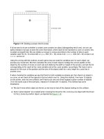
Fig 1.4 shows one example of a 2D coordinate system that we will be discussing again later in the
lesson. It is called the screen coordinate system and it is used to define pixel locations on our viewing
screen. In this case the X axis runs left to right, the Y axis runs from top to bottom, and the origin is
located in the upper left corner.

Figure 1.4

Fig 1.5 shows how four points could be plotted using the screen system and how those points could
have lines drawn between them in series to create a square geometric shape. The polygon looks very
much like one of the polygons in the cube mesh we viewed previously (with the exception that it is
viewed two dimensionally rather than three).

Figure 1.5
www.gameinstitute.com Graphics Programming with DX9
Page 6 of 97


TeamLRN

We must plot these points in a specific sequence so that the line drawing order is clear. We see that a
line should be drawn between point 1 and point 2, and then another between point 2 and point 3 and so
on until we have connected all points and are back at point 1.
It is worth stating that this screen coordinate system is not the preferred design for representing most
two dimensional concepts. First, the Y values increase as the Y axis moves downward. This is contrary
to the common perception that as values increase, they are said to get ‘higher’. Second, the screen
system does not account for a large set of values. In a more complete system, the X and Y axes carry
on to infinity in both positive and negative directions away from the origin (Fig 1.6).

Figure 1.6

Only points within the quadrant of the coordinate system where both X and Y values are positive are
considered valid screen coordinates. Coordinates that fall into any of the other three quadrants are
simply ignored.
Our preferred system will remedy these two concerns. It will reverse the direction of the Y axis such
that increasing values lay out along the upward axis and it will provide the full spectrum of positive
and negative values. This system is the more general (2D) Cartesian coordinate system that most
everyone is familiar with. Fig 1.7 depicts a triangle represented in this standard system:

Figure 1.7

www.gameinstitute.com Graphics Programming with DX9
Page 7 of 97