Hydrological response of watershed systems to land usecover change a case of wami river basin
Bạn đang xem bản rút gọn của tài liệu. Xem và tải ngay bản đầy đủ của tài liệu tại đây (2.05 MB, 10 trang )
Send Orders of Reprints at
78
The Open Hydrology Journal, 2012, 6, 78-87
Open Access
Hydrological Response of Watershed Systems to Land Use/Cover Change.
A Case of Wami River Basin
Joel Nobert* and Jiben Jeremiah
Water Resources Engineering Department, University of Dar es Salaam, Box 35131, Dar es Salaam, Tanzania
Abstract: Wami river basin experiences a lot of human disturbances due to agricultural expansion, and increasing urban
demand for charcoal, fuel wood and timber; resulting in forest and land degradation. Comparatively little is known about
factors that affect runoff behaviour and their relation to landuse in data poor catchments like Wami. This study was conducted to assess the hydrological response of land use/cover change on Wami River flows. In data poor catchments, a
promising way to include landuse change is by integrating Remote Sensing and semi-distributed rainfall-runoff models.
Therefore in this study SWAT model was selected because it applies semi-distributed model domain. Spatial data (landuse, soil and DEM-90m) and Climatic data used were obtained from Water Resources Engineering Department, government offices and from the global data set. SWAT model was used to simulate streamflow for landuse/landcover for the
year 1987 and 2000 to determine the impact of land use/cover change on Wami streamflow after calibrating and validating
with the observed flows. Land use maps of 1987 and 2000 were derived from satellite images using ERDAS Imagine 9.1
software and verified by using 1995 land use which was obtained from Institute of Resource Assessment (IRA).
Findings show that there is decrease of Forest area by 1.4%, a 3.2% increase in Agricultural area, 2.2% increase in Urban
and 0.48% decreases in Waterbody area between 1987 and 2000. The results from SWAT model simulation showed that
the average river flows has decreased from 166.3 mm in 1987 to 165.3 mm in 2000. The surface runoff has increased from
59.4mm (35.7%) in 1987 to 65.9mm (39.9%) in 2000 and the base flow decreased from 106.8mm (64.3%) to 99.4mm
(60.1%) in 1987 and 2000 respectively. This entails that the increase of surface runoff and decrease of base flows are associated with the land use change.
Keywords: Landuse/Landcover change, Hydrological response, Data poor catchments.
1. INTRODUCTION
During recent decades, concerns about the impacts of
changing patterns of landuse associated with deforestation
and agricultural transformation on water resources have created social and political tensions from local to national levels. This shift towards an increasingly urbanized landscape
has generated a number of changes in ecosystem structure
and function, resulting in an overall degradation of the ecological services provided by the natural system in Wami
river basin. Ecosystem services are defined as the multiple
benefits available to humans, animals and plants that are
derived from environmental processes and natural resources
([1] Costanza et al. 1997). Ecosystem services provided by
surface water systems are vital to the health and success of
human development. For example, many urban areas depend
heavily on streams to provide water for municipal, agricultural and commercial uses ([2] Meyer et al. 2005).
Threats to the Ukaguru Mountain forest in Wami river
basin include encroachment from farmers and the plantation
forest, fuel-wood collection and fires spreading from lowland areas. There is a high level of destruction of the forests
in the Nguru Mountains, which have more than 40 endemic
*Address correspondence to this author at the University of Dar es Salaam,
Water Resources Engineering Department, Tanzania; Tel: +255-222410029;
Fax: +255-222410029; E-mail:
1874-3781/12
species. The threats to the Nguru forests are agricultural encroachment and under planting of forest with cardamom and
banana, pit sawing of timber and fires. Other disturbances
include timber harvesting; livestock grazing; pole cutting;
firewood collection and charcoal production ([3] Doggart
and Loserian 2007). Doggart and Loserian (2007) state that
the level of disturbance caused by cardamom cultivation,
hunting and timber harvesting has reached critical levels and
urgent action is needed.
Identifying and quantifying the hydrological consequences of land-use change are not trivial exercises, and are
complicated by: (1) the relatively short lengths of hydrological records; (2) the relatively high natural variability of most
hydrological systems; (3) the difficulties in ‘controlling’
land-use changes in real catchments within which changes
are occurring; (4) the relatively small number of controlled
small-scale experimental studies that have been performed;
and (5) the challenges involved in extrapolating or generalizing results from such studies to other systems. Much of our
present understanding of land-use effects on hydrology is
derived from controlled, experimental manipulations of the
land surface, coupled with pre- and post-manipulation observations of hydrological processes, commonly precipitation
inputs and stream discharge outputs.
In order to account for the natural heterogeneity within
watersheds as well as anthropogenic activities, hydrologic
simulation models are often employed as watershed man2012 Bentham Open
Hydrological Response of Watershed Systems to Land Use/Cover Change
The Open Hydrology Journal, 2012, Volume 6
79
WAMI RIVER SUB-BASIN
KOHDOA
K
K I T E T O
I
L
I
N
D
I
H A N D E N I
K O N G W A
T A N Z A N I A
LEGENDS:
Catchment Boundary
Regional Boundary
District Boundary
Towns
0
50 um
Fig. (1). Wami Sub-basin ([10] WRBWO 2007a).
agement tools. Simulation models have proven useful for
planning managers as a form of decision support for evaluating urbanized watersheds. While conservation efforts have
often focused on maximizing the quantity of land conserved,
research efforts in landscape ecology have shown that the
spatial pattern of land conversion can have a significant effect on the function of ecological processes, particularly
when examining watershed networks. Recently, many research efforts have been launched to predict the hydrologic
response of varying scenarios of land use modification
through the development and application of multiple models
([4] Im et al. 2009). Current models vary tremendously in
their degree of complexity and can range from statistical
simulations, such as a regression analysis or the Spatially
Referenced Regressions on Watershed Attributes (SPARROW) ([5] Schwarz et al. 2006) model, to more processbased models, such as the Soil and Water Assessment Tool
(SWAT) ([6] Neitsch et al. 2005a) or the Hydrologic Simulation Program Fortran (HSPF) ([7] U.S. EPA 1997). In data
poor basins, a promising way to include landuse change is by
integrating Remote Sensing and semi-distributed rainfallrunoff models. Therefore in this study SWAT model was
selected because it applies semi-distributed model domain.
2. DESCRIPTION OF THE STUDY AREA
From its source in the Eastern Arc Mountain ranges of
Tanzania, the Wami River flows in a south-eastwardly direction from dense forests, across fertile agricultural plains and
through grassland savannahs along its course to the Indian
Ocean. Located between 5°–7°S and 36°–39°E, the Wami
River Sub-Basin extends from the semi-arid Dodoma region
to the humid inland swamps in the Morogoro region to
Saadani Village in the coastal Bagamoyo district. It encompasses an area of approximately 43,000 km2 and spans an
altitudinal gradient of approximately 2260 meters (Fig. 1).
According to a 2002 census, the sub-basin is home to 1.8
million people in 12 districts: Kondoa, Dodoma-urban, Bahi,
Chamwino, Kongwa, Mpwapwa, (Dodoma Region) Kiteto,
Simanjiro (Manyara Region), Mvomero, Kilosa (Morogoro
Region), Handeni, Kilindi, (Tanga Region) and Bagamoyo
(Coast Region). It also comprises one of the world’s most
important hotspots of biological diversity: the Eastern Arc
Mountains and coastal forests ([8] WRBWO 2008a).
Average annual rainfall across the Wami sub-basin is estimated to be 550–750 mm in the highlands near Dodoma,
900–1000 mm in the middle areas near Dakawa and 900–
1000 mm at the river’s estuary. Most areas of the Wami sub-
80 The Open Hydrology Journal, 2012, Volume 6
Nobert and Jeremiah
Gra
a
iny
te K
M
IGA1A
Lu
IGD33
ki
e
we
gu
al
ra
IGD16
ya
Tam
IGD14
IG
we
D2
9
do
ng
Lu
m
um
a
IGD31
M
du
kw
e
IG5A
M
IG1
IG6
W
am
i
Kisangata
a
IGD31
i
on
sn
Wami
IG2
ko
nd
IGD56
oa
IGD2
M iy o m
bo
ata
in
Mk
K
IGB1A
Mk
ng
a
iw
sn
en
D
eK
iny
a
gwe
ttl
snn
Li
as
Fig. (2). Schematic representation of the river network ([11] WRBWO 2007d).
basin experience marked differences in rainfall between wet
and dry seasons. Although there is some inter-annual variation in timing of rainfall, dry periods typically occur from
July to October and wet periods from November to December (vuli rains) and from March to June (masika rains) ([9]
WRBWO 2007b). The river network in the Wami sub-basin
drains mainly the arid tract of Dodoma, the central mountains of Rubeho and Nguu and the northern Nguru Mountains. The Wami subbasin river network (WRBWO 2008a)
comprises the main Wami River and its five major tributaries—Lukigura, Diwale, Tami, Mvumi/Kisangata and Mkata
(Fig. 2). The Mkata tributary is the largest and includes two
major sub tributaries, the Miyombo and the large Mkondoa.
The Mkondoa River includes the major Kinyasungwe tributary with the Great and Little Kinyasungwe draining the dry
upper catchments in Dodoma.
3. METHODOLOGY
3.1 SWAT Model
The Soil and Water Assessment Tool (SWAT) is a basinscale model that operates on a daily time step to predict the
impact of land use and management practices on water quality within complex catchments ([12] Arnold and Fohrer
2005). Originally developed by Dr. Jeff Arnold for the
USDA Agricultural Research Service, SWAT was chosen
for this study for its focus on modeling the hydrological impacts of land use change, while specifically accounting for
the interactions between regional soil, land use and slope
characteristics ([13] Arnold et al. 1998).
SWAT is a continuous, long-term, distributed parameter
model designed to predict the impact of land management
practices on the hydrology and sediment and contaminant
transport in agricultural watersheds (Arnold et al., 1998).
SWAT subdivides a watershed into subbasins connected by a
stream network, and further delineates HRUs (Hydrologic
Response Units) consisting of unique combinations of land
cover and soils within each subbasin. The model assumes
that there are no interactions among HRUs, and these HRUs
are virtually located within each subbasin. HRUs delineation
minimizes the computational costs of simulations by lumping similar soil and landuse areas into a single unit ([14] Neitsch et al, 2002).
SWAT is able to simulate surface and subsurface flow,
sediment generation and deposition, and nutrient fate and
movement through landscape and river. The present study
focuses only on the hydrological component of the model.
The hydrologic routines within SWAT account for snow
accumulation and melt, vadose zone processes (i.e., infiltration, evaporation, plant uptake, lateral flows, and percolation), and groundwater flows. Surface runoff is estimated
using a modified version of the USDA-SCS curve number
method ([15] USDA-SCS, 1972). A kinematic storage model
is used to predict lateral flow, whereas return flow is simulated by creating a shallow aquifer (Arnold et al., 1998). The
SWAT model has been extensively tested for hydrologic
modelling at different spatial scales.
The data required to run SWAT were collected and included elevation, land use, soil, climatic data and stream
flow information, as detailed in the following section. After
model set-up was completed, the simulation was run and
calibration procedures were used to improve model accuracy. Next, a future land used scenario was created based on
previous land use change for the area and the output from the
future scenario was compared to the current baseline results,
in order to assess the variance in streamflow.
3.2. Data Preparation
Data is the crucial input for the model in hydrological
modelling. Data preparation, analysis and formatting to suit
the required model input is important and has influences on
the model output. The relevant time series data used for this
study included daily rainfall data, stream flows, temperature
(minimum and maximum), relative humidity, wind speed
and solar radiation. Data were collected from the University
of Dar es Salaam (UDSM), Water Resources Engineering
Department (WRED) data base, Ministry of Water at
Ubungo, Wami Ruvu Basin office at Morogoro and Tanzania
Meteorological Authority office (TMA). These data records
Hydrological Response of Watershed Systems to Land Use/Cover Change
The Open Hydrology Journal, 2012, Volume 6
81
Table 1. Available Rainfall Data
S/N
NAME
Start Year
End Year
Length of Years
Elevation (a.m.s.l)
%Missing
1
9635001
1/1/1932
31/12/1995
64
1120
26.05
2
9536004
1/1/1962
31/12/1991
30
1524
11.00
3
9636029
1/1/1972
31/12/1990
19
914
8.02
4
9635012
1/1/1961
31/12/1990
30
1133
18.03
5
9636008
1/1/1947
31/12/1995
49
1067
27.03
6
9636018
1/1/1956
31/12/1995
40
1676
34.03
7
9635014
1/1/1962
31/12/1995
34
1067
20.07
8
9636013
1/1/1953
31/12/1995
43
914
41.10
9
9736007
1/1/1960
31/12/1989
30
1783
10.17
10
9636027
1/1/1970
31/12/1993
24
1880
12.53
11
9636026
1/1/1970
31/12/1989
20
1786
15.57
12
9536000
1/1/1925
31/12/1961
37
1037
21.97
13
9537009
1/1/1976
31/12/1994
19
1150
52.12
Fig. (3). Temporal distribution of available rainfall data.
Table 2. Climatic and Flow Data
Station Code
Variables
Start Year
End Year
Number of Years
9635001
Relative humidity
1974
1984
10
Wind speed
1974
1984
10
Solar radiation
1974
1984
10
Max and Min temperature
1974
1984
10
Flow
1974
1984
10
1G2
differ in length from the starting and ending dates (Table 1 &
Fig. 3). The selection of the time series data was performed
on the basis of availability and quality of data.
Flow data at the outlet of subbasin (1G2) were used for
calibration purpose. Table 2 shows the climatic data and
flow data used for this study.
Spatial data used included land use data from 30m Landsat TM Satellite, Digital Elevation Model (DEM) with 90-m
resolution and Soil data from Soil and Terrain Database for
Southern Africa (SOTERSAF).
3.3. Model Set-Up
3.3.1. Watershed Delineation
The watershed delineation interface in ArcView
(AVSWAT) is separated into five sections including DEM
Set Up, Stream Definition, Outlet and Inlet Definition, Wa-
82 The Open Hydrology Journal, 2012, Volume 6
Nobert and Jeremiah
N
W
E
S
1GA2
1GB1A
1GD16
1GD14
1G2
1G1
1GD2
Legend
Flow_stations
Rainfall_stations
Rivers
0 20 40
80
120
160
Kilometers
Boundary
subbasins_wami
Fig. (4). Delineated Wami catchment.
tershed Outlet(s) Selection and Definition and Calculation of
Subbasin parameters. In order to delineate the networks subbasins, a critical threshold value is required to define the
minimum drainage area required to form the origin of a
stream.
After the initial subbasin delineation, the generated
stream network can be edited and refined by the inclusion of
additional subbasin inlet or outlets. Adding an outlet at the
location of established monitoring stations is useful for the
comparison of flow concentrations between the predicted and
observed data. Therefore, one subbasin outlet was manually
edited into the watershed based on known stream gage location that had sufficient stream flow data available from 19741984. The delineated catchment is shown in Fig. (4).
3.3.2 HRU Definition
The SWAT (ArcView version) model requires the creation of Hydrologic Response Units (HRUs), which are the
unique combinations of land use and soil type within each
subbasin. The land use and soil classifications for the model
are slightly different than those used in many readily available datasets and therefore the landuse and soil data were
reclassified into SWAT land use and soil classes prior to
running the simulation.
3.4. Land Use Change Analysis
Land use/cover classification was derived from Landsat
satellite images of two different years 1987 and 2000. Supervised classification using ERDAS Imagine software was
used and the final classification resulted into four land cover
classes namely forest, agriculture, water bodies, and urban
areas. The procedure used for the classification of the satellite images and the classified maps are shown in Figs. (5 &
6), respectively. These images were verified by using the
existing landuse/ landcover map of 1995 which was prepared
by Institute of Resource Assessment (IRA) through the
ground truthing.
3.5. Calibration/Sensitivity Analysis
The time series of discharge at the outlet of the catchment
(1G2) was used as data for calibration and validation for
SWAT model, the model was calibrated using the measurements from 1974 to 1980 and first the sensitive parameters
which govern the watershed were obtained and ranked according to their sensitivity (Table 3). The parameters were
optimized first using the auto calibration tool, then calibration was done by adjusting parameters until the simulated
and observed value showed good agreement.
3.6. Model Efficiency Criteria
Nash-Sutcliffe Efficiency (NSE)
The Nash-Sutcliffe efficiency (NSE) is a normalized statistic that determines the relative magnitude of the residual
variance (“noise”) compared to the measured data variance
(“information”) ([16] Nash and Sutcliffe, 1970). NSE indicates how well the plot of observed versus simulated data fits
the 1:1 line. NSE is computed as shown below.
Hydrological Response of Watershed Systems to Land Use/Cover Change
1987 Landsat
bands
Reprojected
Landsat scenes
Stack,
reprojected
and mosaic
Subset
2000 Landsat
bands
Create wami
Basin boundary
Reprojectand
create AOI
1987 and 2000
study area scenes
Radiometic
enhancement
Wami
Basin area
Change maps
and statistics
Cross-tabulation
Vector LU/LC
maps of 1987
and 2000
Dissolve remnant
clouds, delineate
other land uses,
map dicing
Cloud
removal
Vectorise map
chips, dissolve
attributes and
merge vector
chips
Error
assessment,
signature
editing
Map s statistics
The Open Hydrology Journal, 2012, Volume 6
Enhanced images
Image
Interpretation &
creating
classification
scheme
Sampling
training sites
Forest, open
LU/LC,
waterbodies
Supervised
classification
In-process
error
checking
1987 & 2000
signature
Distance rasters
or 1987 and 2000
classifications
Fig. (5). Flowchart for the classification of the satellite images.
Fig. (6). Land use/land cover classifications for the year 1987 (left) and 2000 (right).
Table 3. Sensitivity Ranking of the Parameters
Parameters
Symbol
Rank
CN2
1
SURLAG
2
ESCO
3
ALPHA_BF
4
SOL_Z
5
SOL_AWC
6
Sol_K
7
Effective hydraulic conductivity in main channel alluvium
CH_K2
8
Maximum canopy index
Canmx
9
GWQMN
10
GW_REVAP
11
SCS runoff curve number
Surface runoff lag time(days)
Soil Evaporation Compensation Factor
Base flow Alpha Factor (days)
Soil Depth(m)
Available water capacity
Saturated hydraulic conductivity
Threshold water depth in the shallow aquifer for flow
Ground Water revap coefficient
83
84 The Open Hydrology Journal, 2012, Volume 6
Nobert and Jeremiah
Table 4. Land Use Change Summary
Land Cover Area (km2)
Land cover
Area Change (km2)
Percentage Area
Change (%)
Year 1987
Year 1995
Year 2000
1987_1995
1987_2000
1987_2000
Agricultural area
16527.58
16815.33
16916.68
287.75
389.12
3.17
Forest area
19092.57
18799.33
18655.62
-293.25
-459.77
-1.36
Water Bodies
1020.23
1019.01
994.91
-1.22
-2.53
- 0.48
Urban Area
3359.62
3366.33
3432.79
6.72
73.18
2.23
Total
40000
40000
40000
0
0
4
Agricultural area
Forest area
3
% Area change
Water Bodies
Urban Area
2
1
0
-1
Land cover type
-2
Fig. (7). Percentage of land use/cover change between 1987 and 2000.
2 &
# n
obs
sim
% " Yi ! Yi
(
i=1
(
NSE = 1 ! % n
%
2 (
obs
mean
% " Yi ! Y
(
$ i=1
'
(
)
(
)
Where Yi obs is the i- th observation for the constituent being
evaluated, Yi sim is the i- th simulated value for the constituent
being evaluated, Ymean is the mean of observed data for the
constituent being evaluated, and n is the total number of observations.
NSE ranges between " ! and 1.0 (1 inclusive), with
NSE = 1 being the optimal value. Values between 0.0 and
1.0 are generally viewed as acceptable levels of performance, whereas values <0.0 indicates that the mean observed
value is a better predictor than the simulated value, which
indicates unacceptable performance.
Index of Volumetric Fit (IVF)
Index of Volumetric Fit (IVF) is the ratio of the total estimated volume Qs, to the total observed volume Qo, and is
expressed as.
N
IVF =
! (Q )
i=1
N
!(
i=1
Where
s
Qo
i
)
i
IVF is the Index of Volumetric Fit
(QS )i is volume of the estimated flow
(Qo) is total volume of observed flow
3.7. Analysis of Impact of Landuse/Cover Change on
Streamflows
Three scenarios were used for the analysis of impact of
landuse/cover change on streamflows. In the first scenario
the land use/cover for 1995 was used for calibration and
validation of the model. In the second and third scenarios
land use maps for the year 1987 and 2000, respectively, were
used to simulate the impact of landuse change on streamflows. Hydrological characteristics that were studied and
compared were surface runoff and ground water (base flow)
components.
4. RESULTS AND DISCUSSIONS
4.1. Landuse/Cover Change Analysis
The results for landuse/cover change analysis (Table 4 &
Fig. 7) show that between 1987 and 2000 there was an increase of 3.17% in agricultural land, 1.36% decrease of forest, 0.48% decrease of water bodies, and 2.23% increase in
urban areas. The area change between 1987 and 2000 shows
a decrease of forest area and an increase in agricultural area.
The decrease in forest area and increase of agriculture are
interdependent in Wami basin. The activities which caused
Hydrological Response of Watershed Systems to Land Use/Cover Change
The Open Hydrology Journal, 2012, Volume 6
85
Table 5. Long Term Water Balance Simulation Results
Total Water Yield (mm)
Base Flow (mm)
Surface Flow (mm)
Actual
169.5
107.2
62.2
SWAT
165.4
102.7
62.6
Observed
Simulatec
Rain
0
5
10
15
20
25
30
35
40
1400
1200
1000
800
600
400
200
0
28/08/197602/10/197706/11/197811/12/197914/01/198118/02/1982
Time (Days)
Fig. (8). Calibration Results at the subbasin outlet 1G2 for the land use map of the year 1995.
Observed
Simulated87
1400
Flow(Cumecs)
1200
1000
800
600
400
200
0
28/8/76
10/1/78
25/5/79
6/10/80
18/2/82
Time (Days)
Fig. (9). Scenario 2: Simulated Hydrograph (land use map 1987)
forest decrease in the basin include the increase in farmland
in order to ensure food security and hence clearing of trees
for farm preparation, expanding settlements to meet population growth and other activities including cutting the forest
for timber, construction materials and charcoal. In some areas of Wami, wetlands have changed into agricultural areas
for rice and maize.
4.2. Model Calibration
The model was first calibrated for water balance and
stream flow for average annual condition. Long-term simulation period from 1974 to 1981 was chosen to simulate the
water balance for 1G2 which is considered the catchment
outlet. The calibration results for the water balance for both
surface and base flow components are shown in Table 5.
Calibration and verification was performed for the periods
from 1977 to 1980 and 1975 to 1976, respectively. Nash and
Sutcliff efficiency criteria (NS), and the Index of Volumetric
Fit (IVF) functions were used to test the model performance.
The Nash and Sutcliff coefficient after calibration was 52.2%
and Index of Volumetric Fit (IVF) was 99%.
The Simulated hydrograph (Fig. 8) shows the trend between
observed and simulated flow during calibration, it can be observed that low flows are well reproduced in most periods.
4.3. Land Use/Cover Change Impact on Streamflows
The results from SWAT model simulation showed that
the average river flows has decreased from 166.3 mm in
1987 to 165.3 mm in 2000. The surface runoff has increased
from 59.4mm (35.7%) in 1987 to 65.9mm (39.9%) in 2000
and the base flow decreased from 106.8mm (64.3%) to
99.4mm (60.1%) in 1987 and 2000 respectively.
From the simulated hydrographs (Figs. 9 & 10) it can be
observed that the change in land use between the years 1987
and 2000 caused an increase in the peak flow because of the
land cover change mainly from forest to agriculture and ur-
86 The Open Hydrology Journal, 2012, Volume 6
Nobert and Jeremiah
Observed
Simulated2000
1400
Flow(Cumecs)
1200
1000
800
600
400
200
0
28/8/7616/3/772/10/7720/4/786/11/7825/5/7377/12/718/6/8014/1/81/ 2/8/81
Time (Days)
Fig. (10). Scenario 3: Simulated Hydrograph (land use map 2000).
ban areas. Analyzing peak flows for the simulated hydrograph, on 24th of April 1979, the peak flows were 1069.5
m3/s, 1193.8 m3/s and 1324.6m3/s for the land use data of
1987, 1995 and 2000, respectively. This trend shows that
there is an increase in magnitude of surface flow which is
directly associated with the change in land use cover type.
The change in landuse has affected the ability of the soil to
retain more water (infiltration capacity) during the rain prior
to direct runoff.
5. CONCLUSIONS
A SWAT hydrological model was developed for analysing effects of land use/land cover changes on the stream
flows. The model gave satisfactory results in terms of simulating observed flows. The study findings has revealed that
the Land cover in Wami basin has changed significantly as a
result of disturbances due to encroachment from farmers,
fuel-wood collection and fires spreading from lowland areas.
Degradation of the catchment has affected the flow characteristics in the basin as observed from increase in surface
runoff and decreasing baseflow.
ACKNOWLEDGEMENT
Applied Training Project (ATP) Nile Basin Initiative
REFERENCES
[1]
[2]
[3]
[4]
[5]
[6]
[7]
The main disadvantage of the SWAT model is the fact
that it models many processes and hence h
as hundreds of parameters and requires many data that
make the calibration process tedious. In order to improve the
performance of the model, it is recommended that more efforts should be put in place in collecting more rainfall data or
rehabilitating the gauging stations which are not functioning
at the moment so as to have good spatial representation of
the rainfall data in the catchment. It is also recommended to
use validated remote sensed data to complement ground
measured data so as to have good spatial representation and
to perform hydrological analysis of longer durations than the
available ground measured data.
CONFLICT OF INTEREST
The author confirms that this article content has no conflicts of interest.
[8]
[9]
[10]
[11]
[12]
Costanza R, d’ Age R, Groot R, et al. The value of the world’s
ecosystem services and national capital. Nature 1997; 387: 253-60.
Meyer JL, Michael J, Paul W, Keith WT. Stream Ecosystem Function in Urbanizing Landscapes. J North Am Benthol Soc 2005; 24
(3): 602- 12.
Doggart N, Loserian D. Eds. South Nguru Mountains: a description
of the biophysical landscape. TFCG Technical Paper No 11. DSM
Tz pp 2007; pp. 1-71.
Im S, Hyeonjun K, Chulgyum K, Cheolhee J. Assessing the Impacts of land use changes on watershed hydrology using MIKE
SHE. Environ Geol 2009; 57: 231-9.
Schwarz GE, Hoos AB, Alexander RB, Smith RA. The SPARROW surface water-quality model: theory, application and user
documentation. Reston, Virginia: U.S. Geol Surve 2006; Available
from: />Neitsch SL, Arnold JG, Kiniry JR, Williams JR. a. Soil and water
assessment tool theoretical documentation, Version 2005. Blackland Research Center, USDA Agricultural Research Service. Temple, Texas 76502.
U.S. Environmental Protection Agency (U.S. EPA). 1997. Center
for Exposure Assessment Modeling. The Hydrologic Simulation
Program – FORTRAN (HSPF): Available from: />Wami/Ruvu Basin Water Office (WRBWO). Business Plan.
Wami/Ruvu Basin Water Office, Morogoro 2008a.
Wami/Ruvu Basin Water Office (WRBWO). b. A Rapid Ecological
Assessment of the Wami River Estuary, Tanzania. Prepared by
Anderson EP, McNally C. Global Water for Sustainability Program, Florida International University 2007.
Wami/Ruvu Basin Water Office (WRBWO). a. Environmental
Flow Assessment (EFA), Wami River Sub-Basin, Tanzania: Socioeconomic component of the Wami River EFA Study. Literature
Review for BBM Workshop. 2007. Wami/Ruvu Basin Water Office, Morogoro 2007.
Wami/Ruvu Basin Water Office (WRBWO). d. Environmental
Flow Assessment (EFA), Wami River Sub-Basin, Tanzania: The
Wami Hydrology. Volume 1 – General Description. Wami/Ruvu
Basin Water Office, Morogoro 2007.
Arnold JG, Fohrer N. SWAT 2000: Current Capabilities and Research Opportunities in Applied Watershed Modeling. Hydrol
Process 2005; 19: 563-72.
Hydrological Response of Watershed Systems to Land Use/Cover Change
[13]
[14]
Arnold JG, Srinivasan R, Muttioh RS, Williams JR. Large area
hydrologic modeling and assessment part i: model development. J
Am Water Resour Assoc 1998; 34 (1): 73-89.
Neitsch S, Arnold AG, Kiniry J, Srinivasan J, Williams J. Soil and
Water Assessment Tool Manual: Version 2000. TR-192. College
Station, Texas: Texas Water Resources Institute 2002.
Received: March 26, 2012
The Open Hydrology Journal, 2012, Volume 6
[15]
[16]
Revised: July 03, 2012
87
USDA-SCS. Hydrology. In national engineering handbook. Washington, DC: USDA-SCS 1972.
Nash JE, Sutcliffe JV. River flow forecasting through conceptual
models. Part 1.a discussion of principles. J Hydrol 1970; 10: 28290.
Accepted: July 20, 2012
© Nobert and Jeremiah; Licensee Bentham Open.
This is an open access article licensed under the terms of the Creative Commons Attribution Non-Commercial License
( which permits unrestricted, non-commercial use, distribution and reproduction in any medium, provided the
work is properly cited.