IT training differential equations an introduction with mathematica (2nd ed ) ross 2010 11 25

Undergraduate Texts in Mathematics
Editors

S. Axler
F.W. Gehring
K.A. Ribet


Undergraduate Texts in Mathematics
Abbott: Understanding Analysis.
Anglin: Mathematics: A Concise History
and Philosophy.
Readings in Mathematics.
Anglin/Lambek: The Heritage of
Thales.
Readings in Mathematics.
Apostol: Introduction to Analytic
Number Theory. Second edition.
Armstrong: Basic Topology.
Armstrong: Groups and Symmetry.
Axler: Linear Algebra Done Right.
Second edition.
Reardon: Limits: A New Approach to
Real Analysis.
Bak!Newman: Complex Analysis.
Second edition.
Banchoff/Wermer: Linear Algebra
Through Geometry. Second edition.
Berberian: A First Course in Real
Analysis.
Bix: Conics and Cubics: A

Concrete Introduction to Algebraic
Curves.
Bremaud: An Introduction to
Probabilistic Modeling.
Bressoud: Factorization and Primality
Testing.
Bressoud: Second Year Calculus.
Readings in Mathematics.
Brickman: Mathematical Introduction
to Linear Programming and Game
Theory.
Browder: Mathematical Analysis:
An Introduction.
Buchmann: Introduction to
Cryptography.
Buskes/van Rooij: Topological Spaces:
From Distance to Neighborhood.
Callahan: The Geometry of Spacetime:
An Introduction to Special and General
Relavitity.
Carter/van Brunt: The LebesgueStieltjes Integral: A Practical
Introduction.
Cederberg: A Course in Modern
Geometries. Second edition.

Childs: A Concrete Introduction to
Higher Algebra. Second edition.
Chung/AitSahlia: Elementary Probability
Theory: With Stochastic Processes and
an Introduction to Mathematical

Finance. Fourth edition.
Cox/Little/O'Shea: Ideals, Varieties,
and Algorithms. Second edition.
Croom: Basic Concepts of Algebraic
Topology.
Curtis: Linear Algebra: An Introductory
Approach. Fourth edition.
Daepp/Gorkin: Reading, Writing, and
Proving: A Closer Look at
Mathematics.
Devlin: The Joy of Sets: Fundamentals
of Contemporary Set Theory.
Second edition.
Dixmier: General Topology.
Driver: Why Math?
Ebbinghaus/Fium/Thomas:
Mathematical Logic. Second edition.
Edgar: Measure, Topology, and Fractal
Geometry.
Elaydi: An Introduction to Difference
Equations. Second edition.
Erdi:ls/Suninyi: Topics in the Theory of
Numbers.
Estep: Practical Analysis in One Variable.
Exner: An Accompaniment to Higher
Mathematics.
Exner: Inside Calculus.
Fine/Rosenberger: The Fundamental
Theory of Algebra.
Fischer: Intermediate Real Analysis.

Flanigan/Kazdan: Calculus Two: Linear
and Nonlinear Functions. Second
edition.
Fleming: Functions of Several Variables.
Second edition.
Foulds: Combinatorial Optimization for
Undergraduates.
Foulds: Optimization Techniques: An
Introduction.
(continued after index)


Clay C. Ross

Differential Equations
An Introduction with Mathematica®
Second Edition

With 88 Figures

~Springer


Clay C. Ross
Department of Mathematics
The University of the South
735 University Avenue
Sewanee, TN 37383
USA

Editorial Board
S. Axler
Mathematics Department
San Francisco State
University
San Francisco, CA 94132
USA

F.W. Gehring
Mathematics Department
East Hali
University of Michigan
Ann Arbor, MI 48109
USA

K.A. Ribet
Mathematics Department
University of California,
Berkeley
Berkeley, CA 947.20-3840
USA

Mathematics Subject Classification (2000): 34-01, 65Lxx
Library of Congress Cataloging-in-Publication Data
Ross, Clay C.
Differential equations : an introduction with Mathematica / Clay C. Ross. - 2nd ed.
p. cm. - (Undergraduate texts in mathematics)
Includes bibliographical references and index.
ISBN 978-1-4419-1941-0

ISBN 978-1-4757-3949-7 (eBook)
DOI 10.1007/978-1-4757-3949-7
1. Differential equations.
QA371.R595 2004
515'.35-dc22
ISBN 978-1-4419-1941-0

2. Mathematica (Computer file)

1. Title.

TI. Series.

2004048203

Printed on acid-free paper.

© 2004, 1995 Spinger Science+Business Media New York
Originally published by Springer Science+ Business Media , loc. in 2004
Softcover reprint of the hardcover lod edition 2004
AII rights reserved. This work may not be translated or copied in whole or in part without the written permission of the publisher Springer Science+Business Media, u.e ,
except for brief excerpts in connection with
reviews or scholarly analysis. Use in connection with any farm of information storage
and retrieval, electronic adaptation, computer software, or by similar or dissimilar methodology now known or hereafter developed is farbidden.
The use in this publication oftrade names, trademarks, service marks, and similar terms,
even if they are not identified as such, is not to be taken as an expressio n of opinion as
to whether or not they are subject to proprietary rights.
(MVY)
9 8 7 6 543 2 1
springeronline.com

SPIN 10963685


This book is dedicated to my parents,
Vera K. and Clay C. Ross,
and to my wife,
Andrea,
with special gratitude to each.


Preface

Goals and Emphasis of the Book
Mathematicians have begun to find productive ways to incorporate computing power
into the mathematics curriculum. There is no attempt here to use computing to avoid
doing differential equations and linear algebra. The goal is to make some first explorations in the subject accessible to students who have had one year of calculus.
Some of the sciences are now using the symbol-manipulative power of Mathematica to make more of their subject accessible. This book is one way of doing so for
differential equations and linear algebra.
I believe that if a student's first exposure to a subject is pleasant and exciting,
then that student will seek out ways to continue the study of the subject. The theory
of differential equations and of linear algebra permeates the discussion. Every topic
is supported by a statement of the theory. But the primary thrust here is obtaining
solutions and information about solutions, rather than proving theorems. There are
other courses where proving theorems is central. The goals of this text are to establish
a solid understanding of the notion of solution, and an appreciation for the confidence
that the theory gives during a search for solutions. Later the student can have the same
confidence while personally developing the theory.
When a study of the book has been completed, many important elementary concepts of differential equations and linear algebra will have been encountered. In
addition, the use of Mathematica makes it possible to analyze problems that are

formidable without computational assistance. Mathematica is an integral part of the
presentation, because in introductory differential equations or linear algebra courses
it is too often true that simple tasks like finding an antiderivative, or finding the roots
of a polynomial of relatively high degree-even when the roots are all rationalcompletely obscure the mathematics that is being studied. The complications encountered in the manual solution of a realistic problem of four first-order linear equations with constant coefficients can totally obscure the beauty and centrality of the
theory. But having Mathematica available to carry out the complicated steps frees
the student to think about what is happening, how the ideas work together, and what
everything means.


VIII

Preface

The text contains many examples. Most are followed immediately by the same
example done in Mathematica. The form of a Mathematica notebook is reproduced
almost exactly so that the student knows what to expect when trying problems by
him/herself. Having solutions by Mathematica included in the text also provides a
sort of encyclopedia of working approaches to doing things in Mathernatica. In addition, each of these examples exists as a real Mathematica notebook that can be
executed, studied, printed out, or modified to do some other problem. Other Mathematica notebooks may be provided by the instructor. Occasionally a problem will
request that new methods be tried, but by the time these occur, students should be
able to write effective Mathematica code of their own.
Mathematica can carry the bulk of the computational burden, but this does not
relieve the student of knowing whether or not what is being done is correct. For that
reason, periodic checking of results is stressed. Often an independent manual calculation will keep a Mathematica calculation safely on course. Mathematica, itself, can
and should do much of the checking, because as the problems get more complex, the
calculations get more and more complicated. A calculation that is internally consistent stands a good chance of being correct when the concepts that are guiding the
process are correct.
Since all of the problems except those that are of a theoretical nature can be
solved and checked in Mathematica, very few of the exercises have answers supplied.
As the student solves the problems in each section, they should save the notebooks

to disk-where they can serve as an answer book and study guide if the solutions
have been properly checked. A Mathematica package is a collection of functions
that are designed to perform certain operations. Several notebooks depend heavily
on a package that has been provided. Most of the packages supplied undertake very
complicated tasks, where the functions are genuinely intimidating, so the code does
not appear in the text of study notebooks.
What Is New in This Edition
The changes are two-fold:
1. Rearrange and restate some topics (Linear algebra has now been gathered into
a separate chapter, and series methods for systems have been eliminated.) Many
typographical errors have been corrected.
2. Completely rewrite, and occasionally expand, the Mathematica code using version 5 of Mathematica.
In addition, since Mathematica now includes a complete and fully on-line Help subsystem, several appendices have been eliminated.
Topics Receiving Lesser Emphasis
The solutions of most differential equations are not simple, so the solutions of such
equations are often examined numerically. We indicate some ways to have Mathematica solve differential equations numerically. Also, properties of a solution are


Preface

IX

often deduced from careful examination of the differential equation itself, but an
extended study of qualitative differential equations must wait for a more advanced
course. The best advice is to use the NDSol ve function when a numerical solution
is required.
Some differential equations have solutions that are very hard to describe either
analytically or numerically because the equations are sensitive to small changes in
the initial values. Chaotic behavior is a topic of great current interest; we present
some examples of such equations, but do not fully develop the concepts.

Acknowledgments

I would like to thank those students and others who read the manuscript for the first
edition, and several science department colleagues for enduring questions and for
responding so kindly.
Reviews of the first edition were received from Professors Matthew Richey,
Margie Hale, Stephen L. Clark, Stan Wagon, and William Sit. Dave Withoff contributed to that edition his expert help on technical aspects of Mathematica programming. Any errors that remain in this edition are solely the responsibility of the author.
Sewanee, Tennessee, USA
November 2003

CLAY C. ROSS


Contents

Preface . . . . . . . . . . . . . . . . . . . . . . . . . . . . . . . . . . . . . . . . . . . . . . . . . . . . . . . . . . . . VII
1

About Differential Equations ................................... .
1.0 Introduction . . . . . . . . . . . . . . . . . . . . . . . . . . . . . . . . . . . . . . . . . . . . . . .
1.1 Numerical Methods . . . . . . . . . . . . . . . . . . . . . . . . . . . . . . . . . . . . . . . . .
1.2 Uniqueness Considerations . . . . . . . . . . . . . . . . . . . . . . . . . . . . . . . . . .
1.3 Differential Inclusions (Optional) . . . . . . . . . . . . . . . . . . . . . . . . . . . . .

1
8
17
22

2

Linear Algebra . . . . . . . . . . . . . . . . . . . . . . . . . . . . . . . . . . . . . . . . . . . . . . . .
2.0 Introduction . . . . . . . . . . . . . . . . . . . . . . . . . . . . . . . . . . . . . . . . . . . . . . .
2.1 Familiar Linear Spaces . . . . . . . . . . . . . . . . . . . . . . . . . . . . . . . . . . . . . .
2.2 Abstract Linear Spaces . . . . . . . . . . . . . . . . . . . . . . . . . . . . . . . . . . . . . .
2.3 Differential Equations from Solutions . . . . . . . . . . . . . . . . . . . . . . . . .
2.4 Characteristic Value Problems . . . . . . . . . . . . . . . . . . . . . . . . . . . . . . . .

26
26
31
31
44
48

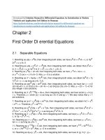
3

First-Order Differential Equations . . . . . . . . . . . . . . . . . . . . . . . . . . . . . . . 52
3.0 Introduction . . . . . . . . . . . . . . . . . . . . . . . . . . . . . . . . . . . . . . . . . . . . . . . 52
3.1 First-Order Linear Differential Equations. . . . . . . . . . . . . . . . . . . . . . . 52
3.2 Linear Equations by M athematica . . . . . . . . . . . . . . . . . . . . . . . . . . . . 57
3.3 Exact Equations............................................ 59
3.4 Variables Separable . . . . . . . . . . . . . . . . . . . . . . . . . . . . . . . . . . . . . . . . . 69
3.5 Homogeneous Nonlinear Differential Equations . . . . . . . . . . . . . . . . . 75
3.6 Bernoulli and Riccati Differential Equations (Optional)........... 79
3.7 Clairaut Differential Equations (Optional) . . . . . . . . . . . . . . . . . . . . . . 86

4

Applications of First-Order Equations. . . . . . . . . . . . . . . . . . . . . . . . . . . . 90

4.0 Introduction . . . . . . . . . . . . . . . . . . . . . . . . . . . . . . . . . . . . . . . . . . . . . . . 90
4.1 Orthogonal Trajectories . . . . . . . . . . . . . . . . . . . . . . . . . . . . . . . . . . . . . 90
4.2 Linear Applications . . . . . . . . . . . . . . . . . . . . . . . . . . . . . . . . . . . . . . . . . 95
4.3 Nonlinear Applications . . . . . . . . . . . . . . . . . . . . . . . . . . . . . . . . . . . . . . 117


XII

Contents

5

Higher-Order Linear Differential Equations . . . . . . . . . . . . . . . . . . . . . .
5.0 Introduction ...............................................
5.1 The Fundamental Theorem ..................................
5.2 Homogeneous Second-Order Linear Constant Coefficients ........
5.3 Higher-Order Constant Coefficients (Homogeneous) .............
5.4 The Method of Undetermined Coefficients .....................
5.5 Variation of Parameters. . . . . . . . . . . . . . . . . . . . . . . . . . . . . . . . . . . . . .

129
129
130
139
152
160
171

6

Applications of Second-Order Equations. . . . . . . . . . . . . . . . . . . . . . . . . .
6.0 Introduction . . . . . . . . . . . . . . . . . . . . . . . . . . . . . . . . . . . . . . . . . . . . . . .
6.1 Simple Harmonic Motion . . . . . . . . . . . . . . . . . . . . . . . . . . . . . . . . . . . .
6.2 Damped Harmonic Motion. . . . . . . . . . . . . . . . . . . . . . . . . . . . . . . . . . .
6.3 Forced Oscillation . . . . . . . . . . . . . . . . . . . . . . . . . . . . . . . . . . . . . . . . . .
6.4 Simple Electronic Circuits . . . . . . . . . . . . . . . . . . . . . . . . . . . . . . . . . . .
6.5 Two Nonlinear Examples (Optional). . . . . . . . . . . . . . . . . . . . . . . . . . .

179
179
179
190
197
202
206

7

The Laplace Transform . . . . . . . . . . . . . . . . . . . . . . . . . . . . . . . . . . . . . . . . .
7.0 Introduction ...............................................
7.1 The Laplace Transform . . . . . . . . . . . . . . . . . . . . . . . . . . . . . . . . . . . . . .
7.2 Properties of the Laplace Transform ...........................
7.3 The Inverse Laplace Transform . . . . . . . . . . . . . . . . . . . . . . . . . . . . . . .
7.4 Discontinous Functions and Their Transforms. . . . . . . . . . . . . . . . . . .

210
210
211
214
225

230

8

Higher-Order Differential Equations with Variable Coefficients . . . . .
8.0 Introduction . . . . . . . . . . . . . . . . . . . . . . . . . . . . . . . . . . . . . . . . . . . . . . .
8.1 Cauchy-Euler Differential Equations ..........................
8.2 Obtaining a Second Solution . . . . . . . . . . . . . . . . . . . . . . . . . . . . . . . . .
8.3 Sums, Products and Recursion Relations . . . . . . . . . . . . . . . . . . . . . . .
8.4 Series Solutions of Differential Equations . . . . . . . . . . . . . . . . . . . . . .
8.5 Series Solutions About Ordinary Points . . . . . . . . . . . . . . . . . . . . . . . .
8.6 Series Solution About Regular Singular Points . . . . . . . . . . . . . . . . . .
8.7 Important Classical Differential Equations and Functions .........

240
240
241
251
253
262
269
277
293

9

Differential Systems: Theory . . . . . . . . . . . . . . . . . . . . . . . . . . . . . . . . . . . .
9.0 Introduction ...............................................
9.1 Reduction to First-Order Systems .............................
9.2 Theory of First-Order Systems ...............................

9.3 First-Order Constant Coefficients Systems . . . . . . . . . . . . . . . . . . . . . .
9.4 Repeated and Complex Roots ................................
9.5 Nonhomogeneous Equations and Boundary-Value Problems ......
9.6 Cauchy-Euler Systems ......................................

297
297
302
309
317
331
344
358


Contents

10

Differential Systems: Applications ...............................
10.0 Introduction ...............................................
10.1 Applications of Systems of Differential Equations ...............
10.2 Phase Portraits ............................................
10.3 Two Nonlinear Examples (Optional) ...........................
10.4 Defective Systems of First-Order Differential
Equations (Optional) ........................................
10.5 Solution of Linear Systems by Laplace Transforms (Optional) .....

XIII

369
369
369
384
404
410
416

References . . . . . . . . . . . . . . . . . . . . . . . . . . . . . . . . . . . . . . . . . . . . . . . . . . . . . . . . . 423
Index ........................................................ ..... 426


1
About Differential Equations

1.0 Introduction
What Are Differential Equations? Who Uses Them?

The subject of differential equations is large, diverse, powerful, useful, and full of
surprises. Differential equations can be studied on their own-just because they are
intrinsically interesting. Or, they may be studied by a physicist, engineer, biologist,
economist, physician, or political scientist because they can model (quantitatively
explain) many physical or abstract systems. Just what is a differential equation? A
differential equation having y as the dependent variable (unknown function) and x as
the independent variable has the form
F(x,y,

~~' ... , ~;) = 0

for some positive integer n. (If n is 0, the equation is an algebraic or transcendental

equation, rather than a differential equation.) Here is the same idea in words:
Definition 1.1. A differential equation is an equation that relates in a nontrivial
manner an unknown function and one or more of the derivatives or differentials of
that unknown function with respect to one or more independent variables.

The phrase "in a nontrivial manner" is added because some equations that appear
to satisfy the above definition are really identities. That is, they are always true, no
matter what the unknown function might be. An example of such an equation is:
. (dy)
dx = 1.
dx + cos2 (dy)
sm2
This equation is satisfied by every differentiable function of one variable. Another
example is:
2
2
( dy
dx + y 2 ·
dx - 2y (dy)
dx - y ) = (dy)

C. C. Ross, Differential Equations
© Springer Science+Business Media New York 2004


2

I About Differential Equations

This is clearly just the binomial squaring rule in disguise: (a+ b) 2 = a:! + 2ab + b2 ;

it, too, is satisfied by every differentiable function of one variable. We want to avoid
calling such identities differential equations.
One quick test to see that an equation is not merely an identity is to substitute
some function such as sin(x) or ex into the equation. If the result is ever false, then
the equation is not an identity and is perhaps worthy of our study. For example,
substitute y = sin(x) into y' + y = 0. The result is cos(x) + sin(x) = 0, and this is
not identically true. (It is false when x = n, for instance.) If you have a complicated
function and are unsure whether or not it is identically 0, you can use Mathematica
to plot the function to see if it ever departs from 0. This does not constitute a proof,
but it is evidence, and it suggests where to look if the function is not identically 0. A
plot can be produced this way:
In [ 1]: = Plot [Cos [x] +Sin [x], {x, 0, 27r}];

1

I

0.5
1

2

3

4

5

6

-0.5
-1

Note that Pi is the symbol n in disguise. The n symbol can be found in the
Basicinput palette.
Another extreme that we would like to avoid is an equation that is never true for
real functions, such as

(dy)
dx

2

2

+y =-I

No matter what the real differentiable function y is, the left-hand side of the equation is nonnegative and the right-hand side is negative-and this cannot happen. So
the equations we want to study are those that can have some solutions, but not too
many solutions. The meaning of this will become clear as we proceed. Unless stated
otherwise, the solutions we seek will be real.
Classification of Differential Equations
Differential equations are classified in several different ways: ordinary or partial;
linear or nonlinear. There are even special subclassifications: homogeneous or


1.0 Introduction

3

nonhomogeneous; autonomous or nonautonomous; first-order, second-order, ...
, nth-order. Most of these names for the various types have been inherited from
other areas of mathematics, so there is some ambiguity in the meanings. But the
context of any discussion will make clear what a given name means in that context.
There are reasons for these classifications, the primary one being to enable discussions about differential equations to focus on the subject matter in a clear and unambiguous manner. Our attention will be on ordinary differential equations. Some will
be linear, some nonlinear. Some will be first-order, some second-order, and some of
higher order than second. What is the order of a differential equation?
Definition 1.2. The order of a differential equation is the order of the highest derivative that appears (nontrivially) in the equation.

At this early stage in our studies, we need only be able to distinguish ordinary
from partial differential equations. This is easy: a differential equation is an ordinary
differential equation if the only derivatives of the unknown function(s) are ordinary
derivatives, and a differential equation is a partial differential equation if the only
derivatives of the unknown function( s) are partial derivatives.
Example 1.1 Here are some ordinary differential equations:

¥r=l+i

(first-order)

d2

~ +y = 3cos(x)

~

{!y__

dx3 + 3d~

[nonlinear]

(second-order) [linear, nonhomogeneous]

5y - 0 (third-order)

[linear, homogeneous]

Example 1.2 Here are some partial differential equations:

au
ax -- au
ay

(first-order in x andy)
(first-order in t; second-order in x)

a2u + aalu
fhZ
2

= 0

(second-order in X andy)
(second-order)

Solutions of Differential Equations
Definition 1.3. To say that y = g(x) is a solution of the differential equation
F

on an interval I means that

(x, y, ~~· ..., : ; ) = 0


4

About Differential Equations

F(x, g(x), g'(x), ... , g
=0

for every choice of x in the interval I. In other words, a solution, when substituted
into the differential equation, makes the equation identically true for x in/.

Example 1.3 The functiony =e-x is a solution of the differential equationy' +y
because y' + y = -e-x + e-x = 0 for all x.

= 0,
o

To have Mathematica verify this for you, conduct this dialog in an active Mathematica window:
In[21:= Clear[x,y, a]
In[31 := y[x_) = Exp[-x]
Out [ 31 = e x
In [ 4 1 : = y' [X) + y [X)

== 0

Out[41= True

The True that Mathematica returned indicates that y'(x) + y(x) = 0 (always), and
hence we indeed have a solution. It is not necessary to Clear variables regularly, but
if you get some unusual behavior, Clear the names involved, re-define them, and try
the calculation again. Mathematica remembers definitions you may have forgotten,
and these may interfere with a subsequent calculation.
Here are other examples of solutions of ordinary differential equations. They are
from the notebook Solutions of DE's. You should execute ideas such as these yourself
in Mathematica.
In [51:= y[x_] = c Exp [x 2 ]
Out[51=

C
X"

In[61 := Simplify[y' [x]- 2xy[x] == 0]
Out[61= True
In[71 := Clear[y]
In[81:= y[t_] =cl Sin[at] +c2 Cos[at]
Out[81= c2 Cos[at] +cl Sin[at]
In[91 := Simplify[y"[t] +a 2 y[t) ==

0]

Out[91= True

Direction Fields and Solutions
The solutions of the first-order differential equation dyl dx = f(x, y) can be represented nicely by a picture. Given a point P = (x, y), the differential equation tells

what the slope of the tangent line to a solution is at the point P. If m is such a slope
then the differential equation says that
m

. y).
-- = f(P) = J(x,
= --'dyl
dx

p


1.0 Introduction

3 I I I '- \ \ I I

2

0

-1

I I I
I I I
I I I
I I I
I I I
I I I
I I I
I I I

I I I
I I I
I I I

\ \ I
/
\ \ \ I
/ '- \ \ \
I-\ \ \
I /'-. \ \
I I - '- \
I I /-'.
I I I /I I I / /
I I I I I
I I I I I

I I I I
I I I I
I I I I
I I I I

-2

I I I I
I I I I
\ I I \
\ I \ I
\ \ \ \
\ \ \ \
\ \ \ \

-.. \

I
I
I
I

\

I
I
I
I
I

I I
I I
I I
I I
I \
\ \ I
\ \ \ \
\ \ \ \
I
I
I
I
\
I

___
' ' ,' ,\. ,\. ,\. ,\ ,\ ,\ ,\ ,\ ,\
//~---------

I I I

I I I
I I I
I I I

- 1

\

I I I I
I I I I
I I I I
I I \ I
I \ \ I
\ I \ I
\ \ \ \
\ \ \ \ \ \

5

0

I

/

/

/

/

I
I
I
I

I
I
I
I

I
I
I
I

I
I
I
I

I I I I I I
I I I I I I

I I I I I I
I I I I I I

///////

2

I I
I I
I I
I I

3

Fig. 1.1. A portion of the direction field of dyldx = (3/2)- 3y + e- 3xl2 .

The idea of a direction field is similar to that of a vector field, where f(x, y), instead
of giving a vector that is to be associated with (x, y), gives a slope that is to be associated with (x, y). If representatives of these slopes are indicated on a graph at enough
points, some visual indication of the behavior of the solutions of the differential
equation is suggested.
For example, in Figure 1.1 we have plotted some representative members of the
direction field associated with the differential equation dy!dx = (3/2)- 3y + e- 3x12 .
Then in Figure 1.2 some solutions of the differential equation are superimposed on
the direction field . Notice how the direction field gives a sense of the behavior of
the solutions. Solutions may be close together, but they do not cross. You may use
the notebook Direction Field Example to produce similar pictures. These can help
you understand the behavior of the solutions of any differential equation that has the
form dyldx = f(x, y).

How Many Solutions Are There?

Once we understand that some differential equations have solutions, it is natural to
ask several questions. How many solutions can a given differential equation have?
(In general there are many; they may be easy or extremely difficult to find.) When
there are many solutions to choose from, is it possible to select one or more having
certain properties? When, if ever, is there exactly one solution having the properties
we want?


6

I About Differential Equations

3
I
I
I
I
\
\
\ \ \ \ \ \ \ \

2

\ \ \ \ \ \ \
,,,,,,
''
/

/

/

/

//

0
I
I

I

-1
-1

0

2

3

Fig.1.2. The direction field of dyldx = (312)- 3y + e- 3xl2 and some solutions.

We will state and often prove theorems that will provide us with guidance as
we seek answers to questions such as these. Some differential equations courses
are structured so that you are asked to prove theorems yourself. In this text, what is
required of you is not the ability to prove these theorems (though you are encouraged
to prove them if you wish), but rather the ability to understand what the theorems
mean, so that you can apply them and thereby profit from the work others have done
on your behalf. Recall that Sir Isaac Newton 1 said "If it be that I have seen further

than other men, it is because I have stood upon the shoulders of giants." It is upon
the shoulders of Newton, himself a giant, and many others since, that we proceed to
stand in the hopes of seeing further than we otherwise might do.
Here is the first such theorem. It is concerned with a differential equation that has
an additional condition specified (an initial condition), having the form given in this
equation:

{ ¥x = f(x, y)

(1.1)

y(xo) =Yo·

Theorem 1.1 (Existence and Uniqueness). Suppose that the real-valued function
f(x, y) is defined and continuous on the rectangle R = [a, b] X [c, d] in the xy-plane,
1

Sir Isaac Newton (1642-1727), British mathematician and natural philosopher. He, along
with Leibniz, created both the differential and integral calculus. He proposed the fundamentallaws of gravitation, was the first to adequately describe properties of light and color, and
constructed the first reflecting telescope. In his later years, Newton was Warden of the Mint,
where he reformed the coinage of the realm, was President of the Royal Society, and was a
member of Parliament.


1.0 Introduction

7

and that (8/f)y)f(x, y) exists and is continuous throughout R. Suppose further that
(x0, y0 ) is an interior point of R. Then there is an open subinterval (a 1, b 1) of [a, b]

centered on x 0 and exactly one solution of the differential equation dy!dx = f(x, y)
that is defined on the subinterval (a 1, b 1) and passes through the point (x0, y0 ).

This theorem tells us that a large class of differential equations have solutions,
and that these solutions are particularly nice: not only do solutions exist, but if you
specify a particular point through which you would like a solution to pass, then
there is exactly one solution that passes through that point. Two concepts are central
here: existence of a solution (there are solutions) and uniqueness of solutions (there
is exactly one solution having the property we want). Existence says that there is
at least one solution; uniqueness says that there is at most one solution. Together,
they say that there is only one solution. This is important, because if you know that
the problem you are solving has a unique solution, and you find a solution, then
you need look no further: the solution you have is the only solution there is. Of
greater importance to those who apply differential equations is the knowledge that if
a process is governed by a differential equation having a unique solution, then if the
process can be performed at all, there is only one way to perform it.
Consider the differential equation dy!dx = sin(y). Here f(x, y) = sin(y) has a continuous partial derivative with respect toy : cos(y). Given any point in the plane, this
differential equation has a unique solution that passes through the point. However,
the differential equation dyldx = y 213 does not (necessarily) have a unique solution
in the vicinity of any point where y = 0, because (8!8y)(y 213 ) = (2/3)y- 113 which is
not continuous when y = 0.
How does one visualize the concept of uniqueness? In Figures 1.2, 4.4, and 4.5,
you can see portions of various families of curves. It is not hard to imagine that each
point of the plane lies on some solution. Furthermore, the solutions do not seem to
cross one another. This is the idea of uniqueness: through each point there is only
one solution. At any point where two solutions cross, we would not have uniqueness.
Look at Figures 1.5 and 1.9 to see examples where this fails. We primarily study
situations where solutions are unique.
Exercises 1.1. Determine whether or not these equations are differential equations.
Classify the differential equations as being ordinary or partial. State the order of each

differential equation.


I About Differential Equations

8

There follow two columns of equations. In the first column is a differential equation; in the second column is a function or set of functions that is a solution of the
differential equation. Verify that the given functions satisfy the corresponding equations. Do this manually and by Mathematica. Consider c 1, c 2 , and A to be arbitrary
constants.
d2
y(t) = c 1 cos(6t) + c 2 sin(6t)
9. qJ + 36y = 0
dt 2

?

2
10. d + 36y
dt

= 72t + 1

11. d 2 y - 36y
dx 2

=0

d2y
12.-2 -36y= 18x+ 1

dx
13.

¥r = 1 + l

14 au = au

. ax

ay

15. 2au
ax

= 3au
ay

y(t) = c 1 cos(6t) + c2 sin(6t) + 2t +

Y( x)
y(t)

= c I e6x + c2 e- 6x -

" 2

-ft

j_
36

= tan(t)

u(x, y)

= f(x + y); f

u(x, y)

= f(3x + 2y); f

arbitrary and differentiable
arbitrary and differentiable

(h)
a
a + · (h))

16 au -aza2u
. at - ax2

u(x, t ) -_ e -.t 2r ( C l

17. a2u + a2u = 0
ax2 al

u(x, y) = e.tx(c 1 cos(t\.y) + c 2 sin(t\.y))

COS,

Cz Slll

1.1 Numerical Methods
Only a very few differential equations can actually be solved-in the sense that we
can write down an expression for a solution. This is especially true of nonlinear
differential equations. In Chapter 3 we discuss many of the special cases where a
solution can actually be obtained. If we need a solution to a differential equation,
but are unable to obtain a closed-form expression for such a solution, how do we get
useful information about the solution? We may just need a few points that lie on the
solution, or we may need to know where our solution crosses some given curve, or
we may wish to determine a maximum or a minimum on the solution. We need such
information in the absence of a function to evaluate.
There are situations where we have to rely on approximating a solution, rather
than obtaining a solution. Leonhard Euler has observed that the direction fields we


1.1 Numerical Methods

9

saw in the introduction to this chapter can be exploited to give us useful information.Suppose that the equation to solve is dy/dx = f(x, y) and the initial point is
y(x0 ) = y 0 • We want a solution over an interval [a, b] with x 0 = a. Since, when his
small,
y(x +h)- y(x)

h

~ y'(x),

Euler reasoned that we should solve

y(x +h)- y(x) _ f(
( ))
h
x,yx

for
y(x +h) = y(x)

+ h f(x, y(x)).

Then, knowing the solution at (x, y(x)), estimate that the solution will pass through
(x + h, y(x) + h f(x, y(x)). This just says that a solution essentially follows its tangent
line, whose direction is that of the direction field element at (x, y(x)). If h is small,
then this guess, though probably wrong, is nevertheless reasonable. This guessing
process is repeated enough times to estimate the solution over the entire interval
[a, b] by finding ordinates corresponding to x 0 = a, x 1 = x 0 + h, x 2 = x 0 + 2h, ...,
xn = x 0 + nh =b. The technique is called Euler's method. We denote y(xk) by yk, and
produce the data points (x0 , y 0 ), (x 1, y 1), ••• , (xn, Yn) by the following rule:
Given x 0 and y0 , the coordinates of the initial point (x 0 , y0 ), and a small number
h, calculate
X
= X +h
k+ I
k
, for 0 :5 k :5 n - 1.
{
Yk+I = Yk + h f(xk, Yk)
It is worth noting that if h < 0 then xn < · · · < x 1 < x 0 , so the points are formed from
right to left.
Euler's method can easily be used with any reasonable spreadsheet. Many spreadsheets even permit plotting the results. Try doing so.

Here is an example that you can use for comparison purposes.
Example 1.4 Use Euler's method to approximate the solution to
dy
dx

= x + 2y,

y(l)

= 1/2

over the interval from x = 1 to x = 3 in steps of h = 0.1.
Solution. For this problem x 0 = 1 and y0 = 1/2 = 0.5. Since h = 0.1, from
xn = x 0 + n h = 1 + (O.l)n = 3 we find that n = (3 - 1)/(0.1) = 20. The process we
need to iterate (repeat) is
xk+I
Yk+I

=
=
=
=

+ 0.1,
}
+ 0.1 f(xk, Yk)
,
+ 0.1 (xk + 2yk)
0.1 xk + 1.2 yk

xk
Yk
Yk

0

:5

k :5 19.

We stop when n = 19 because the point (x 20 , Y2o) is produced at that step. This gives
us 21 data points. The results follow Ex. 1.4M.


10

1 About Differential Equations

Example 1.4 (M) Implement and use the standard Euler method for solving the
problem of Example 1.4 in Mathematica.
In[l]:= Clear[x,y,h,n]

Declare the initial values:
In [2] := x[O] = 1
y[O] =0.5

h

= 0.1

Note that the subscripts are k and k- 1, rather thank+ 1 and k. Mathematica
needs this change for technical reasons. Declare the values for x andy recursively:
In[3]:= x[k_] :=x[k-1] +h

y[k_] := hx[k -1] + 1.2y[k -1]

The exact solution is:
In[4]:= exact[k_] :=-1/4. -x[k]/2+5/4Exp[2x[k] -2]

Produce a four-column table of values. To produce x 20 and y 20 , we need to let k
go to 20.
In[5] :=mat= Table[{k, x[k], y[k], exact[k] }, {k, 0, 20}];

Now format this table of values (named mat) placing headings on the columns.
mat is a table of numbers. What do they mean? For comparison purposes, the last
column is calculated from the exact solution: y(x) = -1/4- x/2 + (5/4)e 2'-2 . This
means that we didn't do very well. Our final y-values are off by more than 20, an
approximately 31% error. Figure 1.3 is a picture of the comparison.
In[6]:= TableForm [mat,

TableHeadings-+ {None, { "k", xk, yk, "exact"}}]
k

0
1
2
3
4
5
6

Out[6]=
7
8
9
10
11
12
13
14
15

xk
1
1.1
1.2
1.3
1.4
1.5
1.6
1.7
1.8
1.9
2.
2.1
2.2
2.3
2 4
2.5
0

yk
0.5
0.7
0.95
1. 26
1.642
2.1104
2.68248
3.37898
4.22477
5.24973
6.48967
7.9876
9.79513
11.9742
14.599
17.7588

exact
0 5
0.726753
1.01478
1.37765
1. 83193
2.39785
3.10015
3 969
5.04129
6.36206
7.98632

9.98127
12.429
15.4297
19.1058
23.6069
0

0


1.1 Numerical Methods
16
17
Out[6]= 18
19
20

2.6
2.7
2. 8
2.9
3.

21 . 5605
26 .1 326
31.6292
38.235
46 . 172

II

29.1157
35 . 855 1
44 . 0978
54.1765
66.4977

Extract and plot the middle two columns of mat (those under the headings xkand
yk). The list m2 of points extracted requires the use of ListPlot. More about

Tran spos e in the next chapter.
In [7] : = m2 =Transpose [Take [Transpose[mat], {2, 3}]]
Out[?]= {{1 , 0.5} , {1.1 , 0.7}, {1.2 , 0.95}, {1.3, 1.26} ,

{1.4 , 1.642} , {1.5 , 2.1104}, {1.6, 2.682 4 8},
{1.7 , 3 . 37898} , {1.8 , 4.22477}, {1.9, 5 . 2 4 973} ,
{2. , 6.48967} , {2 . 1 , 7.9876}, {2.2, 9.79513} ,
{2.3 , 11.9742}, {2.4, 14 . 599} , {2 .5, 17.7588},
{2.6, 2 1. 5605} , {2.7 , 26.1326}, {2.8, 3 1.6 292},
{2.9 , 38.235}, {3 ., 46.172}}
In [ 8] : = p31 = ListPlot [m2];

40
30
20
10
1.5

2

2.5

3

The plot above by ListP lot of the points in table m2 produced a collection of
dots. These are combined with a plot of the exact solution in Fig. 1.3
The option Pl ot Joined-Hrue in ListPlot connects the dots, as in the
plot below.
At least we can say that our approximate solution tried to climb with the exact
solution. But notice that if the exact solution curves upward, our approximation will
be too small at each step because the tangent line at each point lies below the curve,
thereby making our approximation get progressively worse. We have a systematic
error here. It has manifested itself in the poor approximation that we found. The
problem lies in the fact that once an error has taken us off of the actual solution, the
slope is calculated incorrectly for the next point, and the errors may (and in this case
do) get worse as we proceed.


12

1 About Differential Equations

60
50
40

30
20
10
2. 5

3

Fig. 1.3. A comparison of the exact (solid) and approximate (dots) solutions.

Modifying Euler's Method

Often Euler's method is not as bad as this example makes it appear, and the results
can be improved by taking more steps with a smaller value of h. Can anything be
done to eliminate the systematic error that we observed? To make the solution bend
better, we can incorporate the second derivative of our solution into Euler's method.
But, how can the second derivative be found if we do not know the solution? The
problem is not as great as it might seem-we know the derivative of our solution:
dy/dx = x + 2y,and this enables us to implicitly differentiate dy/dx == x + 2y with
respect to x to find that
d 2y
d
dy
dx 2 = dx (x + 2y) = 1 + 2 dx = 1 + 2(x + 2y).

We can take advantage of this once we recall that one form of Taylor's theorem says
that
y(x +h)= y(x) + hy'(x) + (

~: )y"(x) + ( ~~ )y"'(x) + ···.

Euler's method used only the first two terms, y(x)+hy'(x) = y(x)+hf(x, y(x)). We can
use three terms since we now know the second derivative y"(x). This improves our
results. The new process might be called Euler2 since it uses the second derivative.
We can actually calculate as many derivatives as we wish and make a much more

accurate method. The Euler2 method for the differential equation of Example 1.4,
using h = 0.1, is

1/2 = 0.5


1.1 Numerical Methods

= Yk + (O.I)y~ +

Yk+J

13

(O.il' y~

0.005 + (0.1I)xk + (1.22) Yk
for 0 ::s; k ::s; 19. For this differential equation, using the second derivative required
very little extra work. This may not always be the case.
In general, the calculation of y" (x) requires partial derivatives. For instance,
y"(x)

fxJCx, y(x))
oxf(x, y(x)) + oyf(x, y(x))dy!dx

=

fx(x, y(x)) + fyCx, y(x))f(x, y(x))

This second derivative is easy to calculate in Mathematica.

In[9]:= Clear[y]
In[lO]:= f[x_,y_] :=x+2y
In[ll]:= f2[x_,y_] =oxf[x,y] + (oyf[x,y])f[x,y]
Out[ll]= 1+2 (x+2y)

The third derivative is just as simple.
In [12] := £3 [x_, y_] = Simplify[ox £2 [x, y] + (oy £2 [x, y]) f[x, y]]
Out[l2]= 2+4x+8y

The results given are for the problem of Example 1.4. It is clear that being able
to calculate these higher-order derivatives permits us to produce an Euler method
that has any desired number of terms. In numerical analysis, one learns that using
more terms really does improve the accuracy for normal problems. There the topic
of accuracy of a solution is analyzed in thorough detail.
Here is the new Euler2 method. Notice the new term that has been added.
In[13]:= euler2[{x_,y_}] = {x+h,y+hf[x,y] +

(~2 )f2[x,yJ}

Out[l3]= {0.1+x,y+0.1 (x+2y) +0.005 (1+2 (x+2y))}

This is Euler2 for our problem.
In[14]:= Expand[euler2[{x,y}]]
Out[14]= {0.1+x,0.005+0.llx+l.22y}

Make a table of points using Euler 2 , with x 0 and y 0 known from before.
In[15] := x[O]

=1

y[O] = 0.5
h = 0.1


14

1 About Differential Equations

In [ 16] := e2t

= NestList [euler2,

{x [0], y [0]}, 20]

Out[16]= {{1, 0.5}, {1.1, 0.725}, {1.2, 1.0105}, {1.3, 1.36981},
{1.4, 1.81917}, {1.5, 2.37839}, {1.6, 3.07163},
{1.7, 3.92839}, {1.8, 4.98463}, {1.9, 6.28425},
{2., 7.88079}, {2.1, 9.83956}, {2.2, 12.2403},.
{2.3, 15.1801}, {2.4, 18.7778}, {2.5, 23.1779},
{2.6, 28.557}, {2.7, 35.1305}, {2.8, 43.1612},.
{2.9, 52.9697}, {3., 64.9471}}

Again, Li stP lot could produce a plot of this new approximation. Such a plot
with points joined appears as a portion of Fig. 1.4 .
Runge-Kutta and NDSolve

There is a standard method, called the Runge-Kutta method for its creators, that effectively incorporates terms through the fourth derivative, requires no partial derivatives, and needs only four evaluations of the original function f(x, y) to obtain the
next point. Given that the point (xk, yk) is known, the next point (xk+l' Yk+l) is calculated this way:
Table 1.1. Summary of results of several Euler methods.

I

k xk

0
1
2
3
4
5
6
7
8
9
10
11
12
13
14
15
16
17
18
19
20

1.0
1.1
1.2
1.3

1.4
1.5
1.6
1.7
1.8
1.9
2.0
2.1
2.2
2.3
2.4
2.5
2.6
2.7
2.8
2.9
3.0

I Euler I Euler2 I Euler3 I Euler4 I exact
0.5
0.7
0.95
1.26
1.642
2.1104
2.68248
3.37898
4.22477
5.24973
6.48967

7.9876
9.79513
11.9742
14.599
17.7588
21.5605
26.1326
31.6292
38.235
46.172

0.5
0.725
1.0105
1.36981
1.81917
2.37839
3.07163
3.92839
4.98463
6.28425
7.88079
9.83956
12.2403
15.1801
18.7778
23.1779
28.557
35.1305
43.1612

52.9697
64.9471

0.5
0.72667
1.01457
1.37726
1.83129
2.39689
3.09873
3.96698
5.03848
6.35819
7.98107
9.97422
12.4196
15.4172
19.0895
23.5855
29.0878
35.8189
44.051
54.1162
66.4201

0.5
0.72675
1.01477
1.37763
1.8319

2.39781
3.10009
3.96892
5.04118
6.36191
7.98611
9.98099
12.4286
15.4292
19.1052
23.6061
29.1146
35.8537
44.0959
54.1741
66.4946

0.5
0.726753
1.01478
1.37765
1.83193
2.39785
3.10015
3.969
5.04129
6.36206
7.98632
9.98127
12.429

15.4297
19.1058
23.6069
29.1157
35.8551
44.0978
54.1765
66.4977