Test bank and solution of business statistics ch02 statics key (2)

SM_Ch2.pdf
Chap_02.pdf


Chapter 02 - Descriptive Statistics: Tabular and Graphical Method

CHAPTER 2—Descriptive Statistics: Tabular and Graphical Methods and
Descriptive Analytics
§2.1 CONCEPTS
2.1

Constructing either a frequency or a relative frequency distribution helps identify and quantify
patterns that are not apparent in the raw data.
LO02-01

2.2

Relative frequency of any category is calculated by dividing its frequency by the total number of
observations. Percent frequency is calculated by multiplying relative frequency by 100.
LO02-01

2.3

Answers and examples will vary.
LO02-01

§2.1 METHODS AND APPLICATIONS
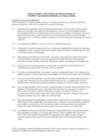
2.4

a.

Test
Response
A
B
C
D

Frequency
100
25
75
50

Relative
Frequency
0.4
0.1
0.3
0.2

Percent
Frequency
40%
10%
30%
20%

b.

Bar Chart of Grade Frequency

120
100
100
75

80
60

50

40

25

20
0
A

B

C

D

LO02-01

2-1
Copyright © 2016 McGraw-Hill Education. All rights reserved. No reproduction or distribution without the prior written consent of McGraw-Hill
Education.

Chapter 02 - Descriptive Statistics: Tabular and Graphical Method

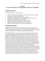
2.5

a.

(100/250) • 360 degrees = 144 degrees for response (a)

b.

(25/250) • 360 degrees = 36 degreesfor response (b)

c.

Pie Chart of Question Response Frequency
D, 50
A, 100

C, 75
B, 25

LO02-01
2.6

a.

Relative frequency for product x is 1 – (0.15 + 0.36 + 0.28) = 0.21

b.

Frequency= relative frequency • N. For W, this is 0.15 • 500 = 75
So we have
product
W
X
Y
Z
frequency

75

105

180

140

c.

Percent Frequency Bar Chart for Product
Preference
36%

40%

28%

30%
20%

21%
15%

10%
0%
W

d.

X

Y

Z

Degrees for W would be 0.15 • 360 = 54; for X: 75.6; for Y: 129.6;
for Z: 100.8.

LO02-01

2-2
Copyright © 2016 McGraw-Hill Education. All rights reserved. No reproduction or distribution without the prior written consent of McGraw-Hill
Education.


Chapter 02 - Descriptive Statistics: Tabular and Graphical Method

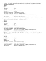
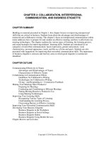
2.7

a.

Rating
Frequency
Outstanding
14
Very Good
10
Good
5
Average
1
Poor
0
∑ = 30

Relative Frequency
14
/30 = 0.467
10
/30 = 0.333
5
/30 = 0.167
1
/30 = 0.033
0
/30 = 0.000

b.

Percent Frequency For Restaurant Rating
50%

47%

40%

33%

30%
17%

20%
10%

3%

0%

0%
Outstanding

Very Good

Good

Average

Poor

c.

Pie Chart For Restaurant Rating
Average, 3%

Poor, 0%

Good,
17%

Very Good,
33%

Outstanding,
47%

LO02-01

2-3
Copyright © 2016 McGraw-Hill Education. All rights reserved. No reproduction or distribution without the prior written consent of McGraw-Hill
Education.


Chapter 02 - Descriptive Statistics: Tabular and Graphical Method

2.8

a.

Frequency Distribution for Sports League Preference

Sports League
MLB
MLS
NBA
NFL
NHL

Frequency
11
3
8
23
5
50

Percent Frequency
0.22
0.06
0.16
0.46
0.10

Percent
22%
6%
16%
46%
10%

b.

Frequency Histogram of Sports League Preference
25

23

20
15
11
10

8
5

5

3

0
MLB

MLS

NBA

NFL

NHL

c.

Frequency Pie Chart of Sports League Preference
NHL N = 50, 0
NHL 5,
0.1
MLB 11, 0.22
MLS 3, 0.06
NFL 23, 0.46

d.

NBA 8, 0.16

The most popular league is NFL and the least popular is MLS.

LO02-011
2-4
Copyright © 2016 McGraw-Hill Education. All rights reserved. No reproduction or distribution without the prior written consent of McGraw-Hill
Education.


Chapter 02 - Descriptive Statistics: Tabular and Graphical Method

2.9

US Market Share in 2005
28.3%

30.0%

26.3%

25.0%
18.3%

20.0%
15.0%

13.6%

13.5%

10.0%
5.0%
0.0%
Chrysler Dodge
Jeep

Ford

GM

Japanese

Other

US Market Share in 2005
Chrysler Dodge
Jeep, 13.6%
Other,

13.5%

Ford, 18.3%

Japanese, 28.3%

GM, 26.3%

LO02-01
2.10 Comparing the pie chart above with chart for 2014 in the textbook shows that between 2005 and
2014, the three U.S. manufacturers, Chrysler, Ford and GM have all lost market share, while
Japanese and other imported models have increased market share.
LO02-01

2-5
Copyright © 2016 McGraw-Hill Education. All rights reserved. No reproduction or distribution without the prior written consent of McGraw-Hill
Education.


Chapter 02 - Descriptive Statistics: Tabular and Graphical Method

2.11 Comparing Types of Health Insurance Coverage Based on Income Level
100%
87%

90%
80%
70%
60%

50%

Income < $30,000

50%
40%

Income > $75,000

33%

30%
17%

20%

9%

10%

4%

0%
Private

Mcaid/Mcare

No Insurance

LO02-01

2-6
Copyright © 2016 McGraw-Hill Education. All rights reserved. No reproduction or distribution without the prior written consent of McGraw-Hill
Education.


Chapter 02 - Descriptive Statistics: Tabular and Graphical Method

2.12 a.

Percent of calls that are require investigation or help = 28.12% + 4.17% =32.29%

b.

Percent of calls that represent a new problem = 4.17%

c.

Only 4% of the calls represent a new problem to all of technical support, but one-third of the
problems require the technician to determine which of several previously known problems this
is and which solutions to apply. It appears that increasing training or improving the
documentation of known problems and solutions will help.

LO02-02

§2.2CONCEPTS
2.13 a.

We construct a frequency distribution and a histogram for a data set so we can gain some
insight into the shape, center, and spread of the data along with whether outliers exist.

b.

A frequency histogram represents the frequencies for the classes using bars while in a
frequency polygon the frequencies are represented by plotted points connected by line
segments.

c.

A frequency ogive represents a cumulative frequency distribution while the frequency polygon
represents a frequency distribution. Also, in a frequency ogive, the points are plotted at the
upper class boundaries; in a frequency polygon, the points are plotted at the class midpoints.

LO02-03
2.14 a.

To find the frequency for a class, you simply count how many of the observations have values
that are greater than or equal to the lower boundary and less than the upper boundary.

b.

Once you determine the frequency for a class, the relative frequency is obtained by dividing
the class frequency by the total number of observations (data points).

c.

The percent frequency for a class is calculated by multiplying the relative frequency by 100.

LO02-03

2-7

Copyright © 2016 McGraw-Hill Education. All rights reserved. No reproduction or distribution without the prior written consent of McGraw-Hill
Education.


Chapter 02 - Descriptive Statistics: Tabular and Graphical Method

2.15 a.

Symmetrical and mound shaped:
One hump in the middle; left side is a mirror image of the right side.

b.

Double peaked:
Two humps, the left of which may or may not look like the right one, nor is each hump
required to be symmetrical

c.

Skewed to the right:
Long tail to the right

d.

Skewed to the left:
Long tail to the left

LO02-03

2-8

Copyright © 2016 McGraw-Hill Education. All rights reserved. No reproduction or distribution without the prior written consent of McGraw-Hill
Education.


Chapter 02 - Descriptive Statistics: Tabular and Graphical Method

§2.2 METHODS AND APPLICATIONS
2.16 a.

Since there are 28 points we use 5 classes (from Table 2.5).

b.

Class Length (CL) = (largest measurement – smallest measurement) / #classes
= (46 – 17) / 5 = 6 (we have rounded up to the integer level since the data
are recorded to the nearest integer.)

c.

The first class’s lower boundary is the smallest measurement, 17.
The first class’s upper boundary is the lower boundary plus the Class Length, 17 + 6 = 23
The second class’s lower boundary is the first class’s upper boundary, 23
Continue adding the Class Length (width) to lower boundaries to obtain the 5 classes:
17 ≤ x<23 | 23 ≤ x< 29 | 29 ≤ x< 35 | 35 ≤ x< 41 | 41 ≤ x ≤ 47

d.

Frequency Distribution for Values
lower
17

23
29
35
41

<
<
<
<
<

upper
23
29
35
41
47

midpoint
20
26
32
38
44

width
6
6
6
6

6

frequency
4
2
4
14
4
28

cumulative
frequency
4
6
10
24
28

percent
14.3
7.1
14.3
50.0
14.3
100.0

cumulative
percent
14.3
21.4

35.7
85.7
100.0

e.
Histogram of Value
14

14
12

Frequency

10
8
6
4

4

4
2

2
0

4

17

23

29

35

41

47

Value

f.

See output in answer to d.

LO02-03
2-9
Copyright © 2016 McGraw-Hill Education. All rights reserved. No reproduction or distribution without the prior written consent of McGraw-Hill
Education.


Chapter 02 - Descriptive Statistics: Tabular and Graphical Method

2-10
Copyright © 2016 McGraw-Hill Education. All rights reserved. No reproduction or distribution without the prior written consent of McGraw-Hill
Education.


Chapter 02 - Descriptive Statistics: Tabular and Graphical Method

2.17 a. and b.Frequency Distribution for Exam Scores
lower
50
60
70
80
90

<
<
<
<
<

upper
60
70
80
90
100

midpoint
55
65
75
85
95

width

10
10
10
10
10

frequency
2
5
14
17
12

percent
4.0
10.0
28.0
34.0
24.0

50

100.0

relative
frequency
0.04
0.10
0.28
0.34

0.24

cumulative
frequency
2
7
21
38
50

cumulative
percent
4.0
14.0
42.0
76.0
100.0

c.
Frequency Polygon
40.0
35.0

Percent

30.0
25.0
20.0
15.0
10.0

5.0
0.0
40

50

60

70

80

90

80

90

Data

d.
Ogive

Cumulative Percent

100.0

75.0

50.0

25.0

0.0
40

50

60

70
Data

LO02-03

2-11
Copyright © 2016 McGraw-Hill Education. All rights reserved. No reproduction or distribution without the prior written consent of McGraw-Hill
Education.


Chapter 02 - Descriptive Statistics: Tabular and Graphical Method

2.18 a.

Because there are 60 data points of design ratings, we use six classes (from Table 2.5).

b.

Class Length (CL) = (Max – Min)/#Classes = (35 – 20) / 6 = 2.5 and we round up to 3, since
the data are recorded to the nearest integer.

c.

The first class’s lower boundary is the smallest measurement, 20.
The first class’s upper boundary is the lower boundary plus the Class Length, 20 + 3 = 23
The second class’s lower boundary is the first class’s upper boundary, 23
Continue adding the Class Length (width) to lower boundaries to obtain the 6 classes:
| 20 < 23 | 23 < 26 | 26 < 29 | 29 < 32 | 32 < 35 | 35 < 38 |

d.

Frequency Distribution for Bottle Design Ratings
lower
20
23
26
29
32
35

<
<
<
<
<
<

upper
23
26

29
32
35
38

midpoint
21.5
24.5
27.5
30.5
33.5
36.5

width
3
3
3
3
3
3

frequency
2
3
9
19
26
1
60

percent
3.3
5
15
31.7
43.3
1.7
100

cumulative
frequency
2
5
14
33
59
60

cumulative
percent
3.3
8.3
23.3
55
98.3
100

e. Distribution shape is skewed left.
Histogram of Rating
26

25

19

Frequency

20

15

9

10

5

3

2
0

20

1
23

26

29
Rating

32

35

38

LO02-03

2-12
Copyright © 2016 McGraw-Hill Education. All rights reserved. No reproduction or distribution without the prior written consent of McGraw-Hill
Education.


Chapter 02 - Descriptive Statistics: Tabular and Graphical Method

Frequency Distribution for Ratings

2.19 a& b.
lower
20
23
26
29
32
35

<
<
<

<
<
<

upper
23
26
29
32
35
38

midpoint
21.5
24.5
27.5
30.5
33.5
36.5

relative
frequency
0.033
0.050
0.150
0.317
0.433
0.017
1.000

width
3
3
3
3
3
3

percent
3.3
5.0
15.0
31.7
43.3
1.7
100

cumulative relative
frequency
0.033
0.083
0.233
0.550
0.983
1.000

cumulative
percent
3.3
8.3

23.3
55.0
98.3
100.0

c.
Ogive

Cumulative Percent

100.0

75.0

50.0

25.0

0.0
17

20

23

26

29

32

35

Rating

LO02-03

2.20 a.

Omitting Dr. Dre leaves us with the annual earnings of 24 celebrities, ranging from 30 to 115
million. We will use five classes (from Table 2.5).
The first class’s lower boundary is the smallest measurement, 30.
Using class length = 18, as prescribed in the problem, the first class’s upper boundary is the
lower boundary plus the class length, 30 + 18 = 48
The second class’s lower boundary is the first class’s upper boundary, 48.
Continue adding the Class Length (width) to lower boundaries to obtain the 5 classes:
| 30<48 | 48<66 | 66<84 |84<102 | 102<120 |
Frequency Distribution for Earnings (omitting Dr. Dre)
lower
30
48
66
84
102

<
<
<
<
<

upper
48
66
84
102
120

midpoint
39
57
75
93
111

width
18
18
18
18
18

frequency
6
8
7
1
2
24

percent
25
33.3
29.2
4.2
8.3
100

cumulative
frequency
6
14
21
22
24

cumulative
percent
25
58.3
87.5
91.7
100

2-13
Copyright © 2016 McGraw-Hill Education. All rights reserved. No reproduction or distribution without the prior written consent of McGraw-Hill
Education.


Chapter 02 - Descriptive Statistics: Tabular and Graphical Method

b. See table in part (a) for cumulative distributions.

c.

d. The first class’s lower boundary is the smallest measurement, 30. Using the suggested class length of
120, the first class’s upper boundary is the lower boundary plus the class length, 30 + 120 = 150
The second class’s lower boundary is the first class’s upper boundary, 150
Continue adding the Class Length (width) to lower boundaries to obtain the 5 classes:
| 30 < 150 | 150 < 270 | 270 < 390 | 390 < 510 | 510 < 630 |
Frequency Distribution for Earnings (including Dr. Dre)
lower
30
150
270
390
510

<
<
<
<
≤

upper
150
270
390
510
630

midpoint
90
210
330
450
570

width
120
120
120
120
120

frequency
24
0
0
0
1
25

percent
96
0
0
0
4
100

cumulative
frequency
24
24
24
24
25

cumulative
percent
96
96
96
96
100

LO02-03
2-14
Copyright © 2016 McGraw-Hill Education. All rights reserved. No reproduction or distribution without the prior written consent of McGraw-Hill
Education.


Chapter 02 - Descriptive Statistics: Tabular and Graphical Method

2.21 a.

The video game satisfaction ratings are concentrated between 40 and 46.

b.

Shape of distribution is slightly skewed left. Recall that these ratings have a minimum value of
7 and a maximum value of 49. This shows that the responses from this survey are reaching
near to the upper limit but significantly diminishing on the low side.

c.

Class:

1
341

Ratings:
d.

CumFreq:

2
364

3
3813

4
4025

5
4245

6
4461

7
4665

LO02-03
2.22 a.

The bank wait times are concentrated between 4 and 9 minutes. (You might make a slightly
different choice.)

b.

The shape of distribution is slightly skewed right. Waiting time has a lower limit of 0 and
stretches out to the high side where there are a few people who have to wait longer.

c.

The class length is 1 minute.

d.

Frequency Distribution for Bank Wait Times

lower
-0.5
0.5
1.5
2.5
3.5
4.5
5.5
6.5
7.5
8.5
9.5
10.5
11.5

<
<
<
<
<
<
<
<
<
<
<
<
<
<

upper
0.5
1.5
2.5
3.5
4.5
5.5
6.5
7.5
8.5
9.5
10.5
11.5
12.5

midpoint
0
1
2
3
4
5
6
7
8
9
10
11
12

width
1
1
1
1
1
1
1
1
1
1
1
1
1

frequency
1
4
7
8
17
16
14
12
8
6
4
2
1
100

percent
1%
4%
7%
8%
17%
16%
14%
12%
8%
6%
4%
2%
1%

cumulative
frequency
1
5
12
20
37
53
67
79
87
93
97
99

100

cumulative
percent
1%
5%
12%
20%
37%
53%
67%
79%
87%
93%
97%
99%
100%

LO02-03

2-15
Copyright © 2016 McGraw-Hill Education. All rights reserved. No reproduction or distribution without the prior written consent of McGraw-Hill
Education.


Chapter 02 - Descriptive Statistics: Tabular and Graphical Method

2.23 a.

The trash bag breaking strengths areconcentrated between 48 and 53 pounds.

b.

The shape of distribution is symmetric and bell shaped.

c.

The class length is 1 pound.

d.

Class:
Cum Freq.

46<47 47<48 48<49 49<50 50<51 51<52 52<53 53<54 54<55
2.5% 5.0% 15.0% 35.0% 60.0% 80.0% 90.0% 97.5% 100.0%
Ogive

Cumulative Percent

100.0

75.0

50.0

25.0

0.0
45

47

49

51

53

Strength

LO02-03

2.24 a.

With 30 values, we will use 5 classes. Note that(Max – Min)/#Classes = (2500 – 485) / 5 =
403. For convenience, we will use classes of length 500 and begin the first class at 250. We
obtain the 5 classes:
| 250 < 750 | 750 < 1250 | 1250 < 1750 | 1750 < 2250 | 2250< 2750 |

Frequency Distribution for MLB Team Values
lower
250
750
1250
1750
2250

<
<

<
<
<

upper
750
1250
1750
2250
2750

midpoint
500
1000
1500
2000
2500

width
500
500
500
500
500

frequency
20
7
1
1

1
30

percent
66.7
23.3
3.3
3.3
3.3
99.9

The distribution is skewed right. While the
majority of teams have valuations under $750
million, a few franchises have much higher
valuations.

2-16
Copyright © 2016 McGraw-Hill Education. All rights reserved. No reproduction or distribution without the prior written consent of McGraw-Hill
Education.


Chapter 02 - Descriptive Statistics: Tabular and Graphical Method

b.

Again, we will use 5 classes. Note that (Max – Min)/#Classes = (461 – 159) / 5 = 60.4. For
convenience, we will use classes of length 75 and begin the first class at 150. We obtain the 5
classes:
| 150 < 225 | 225 < 300 | 300 < 375 | 375 < 450 | 450 < 525 |
Frequency Distribution for MLB Team Revenues

lower
150
225
300
375
450

<
<
<
<
<

upper
225
300
375
450
525

midpoint
187.5
262.5
337.5
412.5
487.5

width
75
75

75
75
75

frequency
17
10
2
0
1
30

percent
56.7
33.3
6.7
0
3.3
100

Histogram of MLB revenues

Frequency

20
15
10
Frequency

5

0
187.5 262.5 337.5 412.5 487.5
revenue class midpoint

c.

percent frequency polygon for MLB team values
80
70
60
50
40

percent

30
20
10
0
0

500 1000 1500 200 2500 3000

2-17
Copyright © 2016 McGraw-Hill Education. All rights reserved. No reproduction or distribution without the prior written consent of McGraw-Hill
Education.


Chapter 02 - Descriptive Statistics: Tabular and Graphical Method

LO02-03
2.25 a. We will use 6 classes since n = 40. Note that (Max – Min)/#Classes = (958 – 57) / 6 = 150.2. For
convenience, we will use classes of length 175 and begin the first class at 0. We obtain the 6
classes:
| 0 < 175 | 175 < 350 | 350 < 525 | 525 < 700 | 700 < 875 | 875 < 1050

Frequency Distribution for Best Small Company Sales
lower
upper midpoint width frequency
0 < 175
87.5
175
9
175 < 350
262.5
175
7
350 < 525
437.5
175
3
525 < 700
612.5
175
6
700 < 875
787.5
175
12
875 < 1050

962.5
175
3
40

Frequency

Frequency histogram for best small company sales, 2014
14
12
10
8
6
4
2
0

Frequency

87.5

262.5 437.5 612.5 787.5 962.5
class midpoints in $millions

b.

We will again use 6 classes. Note that (Max – Min)/#Classes = (75 – 4) / 6 = 11.8. For
convenience, we will use classes of length 15 and begin the first class at 0. We obtain the 6
classes:
| 0 < 15 | 15 < 30 | 30 < 45 | 45 < 60 | 60 < 75 | 75 < 90

Frequency Distribution for Best Small Company Sales Growth
lower
upper midpoint width frequency
0 < 15
7.5
175
16
15 < 30
22.5
175
17
30 < 45
37.5
175
5
45 < 60
52.5
175
1
60 < 75
67.5
175
0
75 < 90
82.5
175
1
2-18

Copyright © 2016 McGraw-Hill Education. All rights reserved. No reproduction or distribution without the prior written consent of McGraw-Hill

Education.


Chapter 02 - Descriptive Statistics: Tabular and Graphical Method

40

Histogram of Best Small Companies Sales Growth

Frequency

20
15
10
Frequency

5
0
7.5

22.5

37.5

52.5

67.5

82.5

Sales growth (%)

LO02-03
2.26 a.

Frequency Distribution for Annual Savings in $000
lower
0
10
25
50
100
150
200
250
500

<
<
<
<
<
<
<
<

upper
10
25
50

100
150
200
250
500

midpoint
5.0
17.5
37.5
75.0
125.0
175.0
225.0
375.0

width
10
15
25
50
50
50
50
250

frequency
162
62
53

60
24
19
22
21
37
460

width =factor
base
10 / 10 =1.0
15 / 10 =1.5
25 / 10 =2.5
50 / 10 =5.0
50 / 10 =5.0
50 / 10 =5.0
50 / 10 =5.0
250 / 10 =25.0

frequency =height
factor
162 / 1.0 =162.0
62 / 1.5 =41.3
53 / 2.5 =21.2
60 / 5.0 =12
24 / 5.0 =4.8
19 / 5.0 =3.8
22 / 5.0 =4.4
21 / 25.0 =0.8

2.26 b. and 2.27
Histogram of Annual Savings in $000
160
150
140
130
120
110
100
90
80
70
60
50
40
30
20
10

162

41.3
21.2
12.0
4.8

3.8

4.4
0.8

0

10

25

50

100

150

200

250

500

* 37

Annual Savings ($000)

2-19
Copyright © 2016 McGraw-Hill Education. All rights reserved. No reproduction or distribution without the prior written consent of McGraw-Hill
Education.


Chapter 02 - Descriptive Statistics: Tabular and Graphical Method

LO02-03

§2.3CONCEPTS
2.28 The horizontal axis spans the range of measurements, and the dots represent the measurements.
LO02-04
2.29 A dot plot with 1,000 points is not practical. Group the data and use a histogram.
LO02-03, LO02-04

§2.3 METHODS AND APPLICATIONS
2.30
DotPlot

0

2

4

6

8

10

12

Absence

The distribution is concentrated between 0 and 2 and is skewed to the right. Eight and ten are
probably high outliers.

LO02-04
2.31
DotPlot

0

0.2

0.4

0.6

0.8

1

Revgrowth

Most growth rates are no more than 71%, but 4 companies had growth rates of 87% or more.
LO02-04
2.32
DotPlot

20

25

30

35

40

45

50

55

60

65

Homers

The distribution is slightly skewed to the left and centered near 45 home runs.
2-20
Copyright © 2016 McGraw-Hill Education. All rights reserved. No reproduction or distribution without the prior written consent of McGraw-Hill
Education.


Chapter 02 - Descriptive Statistics: Tabular and Graphical Method

LO02-04

2-21
Copyright © 2016 McGraw-Hill Education. All rights reserved. No reproduction or distribution without the prior written consent of McGraw-Hill
Education.

Chapter 02 - Descriptive Statistics: Tabular and Graphical Method

§2.4 CONCEPTS
2.33 Both the histogram and the stem-and-leaf show the shape of the distribution, but only the stem-andleaf shows the values of the individual measurements.
LO02-03, LO02-05
2.34 Several advantages of the stem-and-leaf display include that it:
-Displays all the individual measurements.
-Puts data in numerical order
-Is simple to construct
LO02-05
2.35 With a large data set (e.g., 1,000 measurements) it does not make sense to use a stem-and-leaf
because it is impractical to write out 1,000 data points. Group the data and use a histogram.
LO02-03, LO02-05

§2.4 METHODS AND APPLICATIONS
2.36

Stem Unit = 10, Leaf Unit = 1 Revenue Growth in Percent
Frequency
1
4
5
5
2
1
1
1
20

Stem

2
3
4
5
6
7
8
9

Leaf
8
0 2 3 6
2 2 3 4 9
1 3 5 6 9
3 5
0
3
1

LO02-05

2-22
Copyright © 2016 McGraw-Hill Education. All rights reserved. No reproduction or distribution without the prior written consent of McGraw-Hill
Education.


Chapter 02 - Descriptive Statistics: Tabular and Graphical Method

Stem Unit = 1, Leaf Unit =.1 Profit Margins (%)

2.37

Frequency
2
0
1
3
4
4
4
0
0
0
0
0
1
0
0
1
20

Stem
10
11
12
13
14
15
16
17

18
19
20
21
22
23
24
25

Leaf
4 4
6
2
0
2
1

8
1
2
1

9
4 9
8 9
4 8

2
2

LO02-05
Stem Unit = 1000, Leaf Unit = 100 Sales($mil)

2.38

Frequency
5
5
4
2
1
2
1

Stem
1
2
3
4
5
6
7

Leaf
2 4 4 5 7
0 4 7 7 8
3 3 5 7
2 6
4
0 8

9

LO02-05
2.39 a.
b.

The Payment Times distribution is skewed to the right.
The Bottle Design Ratings distribution is skewed to the left.

LO02-05
2.40 a.
b.

The distribution is symmetric and centered near 50.7 pounds.
46.8, 47.5, 48.2, 48.3, 48.5, 48.8, 49.0, 49.2, 49.3, 49.4

LO02-05

2-23
Copyright © 2016 McGraw-Hill Education. All rights reserved. No reproduction or distribution without the prior written consent of McGraw-Hill
Education.


Chapter 02 - Descriptive Statistics: Tabular and Graphical Method

2.41 Stem unit = 10, Leaf Unit = 1
Leaf
Roger Maris
8
6 4 3

8 6 3
9 3
1

Stem
0
1
2
3
4
5
6

Home Runs

Leaf
Babe Ruth
2
4
1
4
0

5
5
1 6 6 6 7 9
4 9

The 61 home runs hit by Maris would be considered an outlier for him, although an exceptional
individual achievement.

LO02-05
2.42 a.

Stem unit = 1, Leaf Unit = 0.1 Bank Customer Wait Time
Frequency
2
6
9
11
17
15
13
10
7
6
3
1
100

b.

Stem
0
1
2
3
4
5
6
7

8
9
10
11

Leaf
4 8
1 3
0 2
1 2
0 0
0 1
1 1
0 2
0 1
1 2
2 7
6

4
3
4
1
1
2
2
3
3
9

6
4
5
2
2
3
3
4
5

8
5
6
3
2
3
4
6
8

8
7
7
3
3
3
4
6
9

8
7
3
4
4
5
7

9
8
4
4
5
7

9
8
4
5
5
8

9
5
6
6
9

9
5 5 6 7 7 8 9

6 7 8 8 8
7 7 8

The distribution of wait times is fairly symmetrical, maybe with a slight skew to the right.

LO02-05

2-24
Copyright © 2016 McGraw-Hill Education. All rights reserved. No reproduction or distribution without the prior written consent of McGraw-Hill
Education.