Test bank and solution manual of descritve statistics (2)

Chapter 02 - Descriptive Statistics: Tabular and Graphical Method

CHAPTER 2—Descriptive Statistics: Tabular and Graphical Methods
§2.1 CONCEPTS
2.1

Constructing either a frequency or a relative frequency distribution helps identify and quantify
patterns that are not apparent in the raw data.
LO02-01

2.2

Relative frequency of any category is calculated by dividing its frequency by the total number of
observations. Percent frequency is calculated by multiplying relative frequency by 100.
LO02-01

2.3

Answers and examples will vary.
LO02-01

§2.1 METHODS AND APPLICATIONS
2.4

a.

Test
Response
A
B
C

D

Frequency
100
25
75
50

Relative
Frequency
0.4
0.1
0.3
0.2

Percent
Frequency
40%
10%
30%
20%

b.

Bar Chart of Grade Frequency
120
100
100
75

80
60

50

40

25

20
0
A

B

C

D

LO02-01

2-1
Copyright © 2015 McGraw-Hill Education. All rights reserved. No reproduction or distribution without the prior written consent of McGraw-Hill
Education.


Chapter 02 - Descriptive Statistics: Tabular and Graphical Method

2.5

a.

(100/250) • 360 degrees = 144 degrees for response (a)

b.

(25/250) • 360 degrees = 36 degrees for response (b)

c.

Pie Chart of Question Response Frequency
D, 50
A, 100

C, 75
B, 25

LO02-01
2.6

a.

Relative frequency for product x is 1 – (0.15 + 0.36 + 0.28) = 0.21

b.

Product:
W X
Y Z
frequency = relative frequency • N = 0.15 • 500 = 75 105 180 140

c.

Percent Frequency Bar Chart for Product
Preference
36%

40%

28%

30%
20%

21%
15%

10%
0%
W

d.

X

Y

Z

Degrees for W would be 0.15 • 360 = 54

for X 75.6
for Y 129.6
for Z 100.8.

LO02-01

2-2
Copyright © 2015 McGraw-Hill Education. All rights reserved. No reproduction or distribution without the prior written consent of McGraw-Hill
Education.


Chapter 02 - Descriptive Statistics: Tabular and Graphical Method

2.7

a.

Rating
Outstanding
Very Good
Good
Average
Poor

Frequency
14
10
5
1
0

∑ = 30

Relative Frequency
14
/30 = 0.467
10
/30 = 0.333
5
/30 = 0.167
1
/30 = 0.033
0
/30 = 0.000

b.

Percent Frequency For Restaurant Rating
50%

47%

40%

33%

30%
17%

20%
10%

3%

0%

0%
Outstanding

Very Good

Good

Average

Poor

c.

Pie Chart For Restaurant Rating
Average, 3%

Poor, 0%

Good,
17%

Very Good,
33%

Outstanding,

47%

LO02-01

2-3
Copyright © 2015 McGraw-Hill Education. All rights reserved. No reproduction or distribution without the prior written consent of McGraw-Hill
Education.


Chapter 02 - Descriptive Statistics: Tabular and Graphical Method

2.8

a.

Frequency Distribution for Sports League Preference
Sports League
MLB
MLS
NBA
NFL
NHL

Frequency
11
3
8
23
5
50

Percent Frequency
0.22
0.06
0.16
0.46
0.10

Percent
22%
6%
16%
46%
10%

b.

Frequency Histogram of Sports League Preference
25

23

20
15
11
10

8
5

5

3

0
MLB

MLS

NBA

NFL

NHL

c.

Frequency Pie Chart of Sports League Preference
NHL N = 50, 0
NHL 5,
0.1
MLB 11, 0.22
MLS 3, 0.06
NFL 23, 0.46

d.

NBA 8, 0.16

The most popular league is NFL and the least popular is MLS.

LO02-011

2-4
Copyright © 2015 McGraw-Hill Education. All rights reserved. No reproduction or distribution without the prior written consent of McGraw-Hill
Education.


Chapter 02 - Descriptive Statistics: Tabular and Graphical Method

2.9

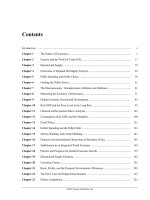
US Market Share in 2005
28.3%

30.0%

26.3%

25.0%
18.3%

20.0%
15.0%

13.6%

13.5%

10.0%

5.0%
0.0%
Chrysler Dodge
Jeep

Ford

GM

Japanese

Other

US Market Share in 2005
Chrysler Dodge
Jeep, 13.6%
Other,
13.5%

Ford, 18.3%

Japanese, 28.3%

GM, 26.3%

LO02-01
2.10 Comparing the pie chart above and the chart for 2010 in the text book shows that between 2005 and
2010, the three U.S. manufacturers, Chrysler, Ford and GM have all lost market share, while
Japanese and other imported models have increased market share.
LO02-01

2-5
Copyright © 2015 McGraw-Hill Education. All rights reserved. No reproduction or distribution without the prior written consent of McGraw-Hill
Education.


Chapter 02 - Descriptive Statistics: Tabular and Graphical Method

2.11 Comparing Types of Health Insurance Coverage Based on Income Level
100%
87%

90%
80%
70%
60%

50%

Income < $30,000

50%
40%

Income > $75,000

33%

30%
17%

20%

9%

10%

4%

0%
Private

Mcaid/Mcare

No Insurance

LO02-01

2-6
Copyright © 2015 McGraw-Hill Education. All rights reserved. No reproduction or distribution without the prior written consent of McGraw-Hill
Education.


Chapter 02 - Descriptive Statistics: Tabular and Graphical Method

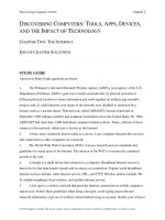
2.12 a.

Percent of calls that are require investigation or help = 28.12% + 4.17% = 32.29%

b.

Percent of calls that represent a new problem = 4.17%

c.

Only 4% of the calls represent a new problem to all of technical support, but one-third of the
problems require the technician to determine which of several previously known problems this
is and which solutions to apply. It appears that increasing training or improving the
documentation of known problems and solutions will help.

LO02-02

§2.2 CONCEPTS
2.13 a.

We construct a frequency distribution and a histogram for a data set so we can gain some
insight into the shape, center, and spread of the data along with whether or not outliers exist.

b.

A frequency histogram represents the frequencies for the classes using bars while in a
frequency polygon the frequencies are represented by plotted points connected by line
segments.

c.

A frequency ogive represents a cumulative distribution while the frequency polygon does not
represent a cumulative distribution. Also, in a frequency ogive, the points are plotted at the
upper class boundaries; in a frequency polygon, the points are plotted at the class midpoints.

LO02-03
2.14 a.

To find the frequency for a class, you simply count how many of the observations have values
that are greater than or equal to the lower boundary and less than the upper boundary.

b.

Once you determine the frequency for a class, the relative frequency is obtained by dividing
the class frequency by the total number of observations (data points).

c.

The percent frequency for a class is calculated by multiplying the relative frequency by 100.

LO02-03

2-7
Copyright © 2015 McGraw-Hill Education. All rights reserved. No reproduction or distribution without the prior written consent of McGraw-Hill
Education.


Chapter 02 - Descriptive Statistics: Tabular and Graphical Method

2.15 a.

Symmetrical and mound shaped:
One hump in the middle; left side is a mirror image of the right side.

b.

Double peaked:
Two humps, the left of which may or may not look like the right one, nor is each hump
required to be symmetrical

c.

Skewed to the Right:
Long tail to the right

d. Skewed to the left:
Long tail to the left

LO02-03

2-8
Copyright © 2015 McGraw-Hill Education. All rights reserved. No reproduction or distribution without the prior written consent of McGraw-Hill
Education.


Chapter 02 - Descriptive Statistics: Tabular and Graphical Method

§2.2 METHODS AND APPLICATIONS
2.16 a.

Since there are 28 points we use 5 classes (from Table 2.5).

b.

Class Length (CL) = (largest measurement – smallest measurement) / #classes

= (46 – 17) / 5 = 6
(If necessary, round up to the same level of precision as the data itself.)

c.

The first class’s lower boundary is the smallest measurement, 17.
The first class’s upper boundary is the lower boundary plus the Class Length, 17 + 3 = 23
The second class’s lower boundary is the first class’s upper boundary, 23
Continue adding the Class Length (width) to lower boundaries to obtain the 5 classes:
17 ≤ x < 23 | 23 ≤ x < 29 | 29 ≤ x < 35 | 35 ≤ x < 41 | 41 ≤ x ≤ 47

d.

Frequency Distribution for Values
lower
17
23
29
35
41

<
<
<
<
<

upper
23
29

35
41
47

midpoint
20
26
32
38
44

width
6
6
6
6
6

frequency
4
2
4
14
4
28

cumulative
frequency
4
6

10
24
28

percent
14.3
7.1
14.3
50.0
14.3
100.0

cumulative
percent
14.3
21.4
35.7
85.7
100.0

e.
Histogram of Value
14

14
12

Frequency

10

8
6
4

4

4
2

2
0

4

17

23

29

35

41

47

Value

f.

See output in answer to d.

LO02-03

2-9
Copyright © 2015 McGraw-Hill Education. All rights reserved. No reproduction or distribution without the prior written consent of McGraw-Hill
Education.


Chapter 02 - Descriptive Statistics: Tabular and Graphical Method

2.17 a. and b. Frequency Distribution for Exam Scores
lower
50
60
70
80
90

<
<
<
<
<

upper
60
70
80
90

100

midpoint
55
65
75
85
95

width
10
10
10
10
10

frequency
2
5
14
17
12

percent
4.0
10.0
28.0
34.0
24.0

50

100.0

relative
frequency
0.04
0.10
0.28
0.34
0.24

cumulative
frequency
2
7
21
38
50

cumulative
percent
4.0
14.0
42.0
76.0
100.0

c.
Frequency Polygon

40.0
35.0

Percent

30.0
25.0
20.0
15.0
10.0
5.0
0.0
40

50

60

70

80

90

80

90

Data

d.
Ogive

Cumulative Percent

100.0

75.0

50.0

25.0

0.0
40

50

60

70
Data

LO02-03

2-10
Copyright © 2015 McGraw-Hill Education. All rights reserved. No reproduction or distribution without the prior written consent of McGraw-Hill
Education.

Chapter 02 - Descriptive Statistics: Tabular and Graphical Method

2.18 a.

Because there are 60 data points of design ratings, we use six classes (from Table 2.5).

b.

Class Length (CL) = (Max – Min)/#Classes = (35 – 20) / 6 = 2.5 and we round up to 3, the
level of precision of the data.

c.

The first class’s lower boundary is the smallest measurement, 20.
The first class’s upper boundary is the lower boundary plus the Class Length, 20 + 3 = 23
The second class’s lower boundary is the first class’s upper boundary, 23
Continue adding the Class Length (width) to lower boundaries to obtain the 6 classes:
| 20 < 23 | 23 < 26 | 26 < 29 | 29 < 32 | 32 < 35 | 35 < 38 |

d.

Frequency Distribution for Bottle Design Ratings
lower
20
23
26
29
32
35

<
<
<
<
<
<

upper
23
26
29
32
35
38

midpoint
21.5
24.5
27.5
30.5
33.5
36.5

width
3
3
3
3
3
3

frequency
2
3
9
19
26
1
60

percent
3.3
5
15
31.7
43.3
1.7
100

cumulative
frequency
2
5
14
33
59
60

cumulative
percent

3.3
8.3
23.3
55
98.3
100

e. Distribution shape is skewed left.
Histogram of Rating
26
25

19

Frequency

20

15

9

10

5

3

2
0

20

1
23

26

29
Rating

32

35

38

LO02-03

2-11
Copyright © 2015 McGraw-Hill Education. All rights reserved. No reproduction or distribution without the prior written consent of McGraw-Hill
Education.


Chapter 02 - Descriptive Statistics: Tabular and Graphical Method

Frequency Distribution for Ratings

2.19 a & b.
lower

20
23
26
29
32
35

<
<
<
<
<
<

upper
23
26
29
32
35
38

midpoint
21.5
24.5
27.5
30.5
33.5
36.5

relative
frequency
0.033
0.050
0.150
0.317
0.433
0.017
1.000

width
3
3
3
3
3
3

percent
3.3
5.0
15.0
31.7
43.3
1.7
100

cumulative relative
frequency
0.033

0.083
0.233
0.550
0.983
1.000

cumulative
percent
3.3
8.3
23.3
55.0
98.3
100.0

c.
Ogive

Cumulative Percent

100.0

75.0

50.0

25.0

0.0
17

20

23

26

29

32

35

Rating

LO02-03
2.20 a.

Because we have the annual pay of 25 celebrities, we use five classes (from Table 2.5).
Class Length (CL) = (290 – 28) / 5 = 52.4 and we round up to 53 since the data are in whole
numbers.
The first class’s lower boundary is the smallest measurement, 28.
The first class’s upper boundary is the lower boundary plus the Class Length, 28 + 53 = 81
The second class’s lower boundary is the first class’s upper boundary, 81
Continue adding the Class Length (width) to lower boundaries to obtain the 5 classes:
| 28 < 81 | 81 < 134 | 134 < 187 | 187 < 240 | 240 < 293 |

2-12
Copyright © 2015 McGraw-Hill Education. All rights reserved. No reproduction or distribution without the prior written consent of McGraw-Hill
Education.

Chapter 02 - Descriptive Statistics: Tabular and Graphical Method

2.20 a. (cont.)
Frequency Distribution for Celebrity Annual Pay($mil)
lower
28
81
134
187
240

<
<
<
<
<
<

upper
81
134
187
240
293

midpoint
54.5
107.5

160.5
213.5
266.5

width
53
53
53
53
53

frequency
17
6
0
1
1
25

percent
34.0
12.0
0.0
2.0
2.0
50.0

cumulative
frequency
17

23
23
24
25

cumulative
percent
34.0
46.0
46.0
48.0
50.0

Histogram of Pay ($mil)
18
16
14

Frequency

12
10
8
6
4
2
0

28

81

134
187
Pay ($mil)

240

293

c.
Ogive

Cumulative Percent

100.0

75.0

50.0

25.0

0.0
28

81

134
187

Pay ($mil)

240

LO02-03

2-13
Copyright © 2015 McGraw-Hill Education. All rights reserved. No reproduction or distribution without the prior written consent of McGraw-Hill
Education.


Chapter 02 - Descriptive Statistics: Tabular and Graphical Method

2.21 a.

The video game satisfaction ratings are concentrated between 40 and 46.

b.

Shape of distribution is slightly skewed left. Recall that these ratings have a minimum value of
7 and a maximum value of 49. This shows that the responses from this survey are reaching
near to the upper limit but significantly diminishing on the low side.

c.

Class:

Ratings:
d.

Cum Freq:

1
341

2
364

3
3813

4
4025

5
4245

6
4461

7
4665

LO02-03
2.22 a.

The bank wait times are concentrated between 4 and 7 minutes.

b.

The shape of distribution is slightly skewed right. Waiting time has a lower limit of 0 and
stretches out to the high side where there are a few people who have to wait longer.

c.

The class length is 1 minute.

d.

Frequency Distribution for Bank Wait Times
lower
-0.5
0.5
1.5
2.5
3.5
4.5
5.5
6.5
7.5
8.5
9.5
10.5

11.5

<
<
<
<
<
<
<
<
<
<
<
<
<
<

upper
0.5
1.5
2.5
3.5
4.5
5.5
6.5
7.5
8.5
9.5
10.5
11.5

12.5

midpoint
0
1
2
3
4
5
6
7
8
9
10
11
12

width
1
1
1
1
1
1
1
1
1
1
1
1

1

frequency
1
4
7
8
17
16
14
12
8
6
4
2
1
100

percent
1%
4%
7%
8%
17%
16%
14%
12%
8%
6%
4%

2%
1%

cumulative
frequency
1
5
12
20
37
53
67
79
87
93
97
99
100

cumulative
percent
1%
5%
12%
20%
37%
53%
67%
79%
87%

93%
97%
99%
100%

LO02-03

2-14
Copyright © 2015 McGraw-Hill Education. All rights reserved. No reproduction or distribution without the prior written consent of McGraw-Hill
Education.


Chapter 02 - Descriptive Statistics: Tabular and Graphical Method

2.23 a.

The trash bag breaking strengths are concentrated between 48 and 53 pounds.

b.

The shape of distribution is symmetric and bell shaped.

c.

The class length is 1 pound.

d.

Class:
Cum Freq.

46<47 47<48 48<49 49<50 50<51 51<52 52<53 53<54 54<55
2.5% 5.0% 15.0% 35.0% 60.0% 80.0% 90.0% 97.5% 100.0%
Ogive

Cumulative Percent

100.0

75.0

50.0

25.0

0.0
45

47

49

51

53

Strength

LO02-03
2.24 a.

Because there are 30 data points, we will use 5 classes (Table 2.5). The class length will be
(1700-304)/5= 279.2, rounded to the same level of precision as the data, 280.
Frequency Distribution for MLB Team Value ($mil)
lower
304
584
864
1144
1424

<
<
<
<
<

upper
584
864
1144
1424
1704

midpoint
444
724
1004
1284
1564

width
280
280
280
280
280

frequency
24
4
1
0
1
30

percent
80.0
13.3
3.3
0.0
3.3
100.0

cumulative
frequency
24
28
29
29

30

cumulative
percent
80.0
93.3
96.7
96.7
100.0

Histogram of Value $mil
25

Frequency

20

15

10

5

0

304

584

864

1144
Value $mil

1424

1704

Distribution is skewed right and has a distinct outlier, the NY Yankees.

2-15
Copyright © 2015 McGraw-Hill Education. All rights reserved. No reproduction or distribution without the prior written consent of McGraw-Hill
Education.


Chapter 02 - Descriptive Statistics: Tabular and Graphical Method

2.24 b.

Frequency Distribution for MLB Team Revenue
lower
143
200
257
314
371

<
<
<
<

<

upper
200
257
314
371
428

midpoint
171.5
228.5
285.5
342.5
399.5

width
57
57
57
57
57

frequency
16
11
2
0
1
30

percent
53.3
36.7
6.7
0.0
3.3
100.0

cumulative
frequency
16
27
29
29
30

cumulative
percent
53.3
90.0
96.7
96.7
100.0

Histogram of Revenues $mil
18
16
14

Frequency

12
10
8
6
4
2
0

143

200

257
314
Revenues $mil

371

428

The distribution is skewed right.

c.
Percent Frequency Polygon
100.0

Percent

80.0
60.0
40.0
20.0
0.0
304

584

864
1,144
Value ($mil)

1,424

LO02-03

2-16
Copyright © 2015 McGraw-Hill Education. All rights reserved. No reproduction or distribution without the prior written consent of McGraw-Hill
Education.


Chapter 02 - Descriptive Statistics: Tabular and Graphical Method

2.25 a.

Because there are 40 data points, we will use 6 classes (Table 2.5). The class length will be
(986-75)/6= 151.83. Rounding up to the same level of precision as the data gives a width of
152. Beginning with the minimum value for the first lower boundary, 75, add the width, 152,
to obtain successive boundaries.

Frequency Distribution for Sales ($mil)
lower
75
227
379
531
683
835

<
<
<
<
<
<

upper
227
379
531
683
835
987

midpoint
151
303
455
607
759

911

width
152
152
152
152
152
152

frequency
9
8
5
7
4
7
40

percent
22.5
20.0
12.5
17.5
10.0
17.5
100.0

cumulative
frequency

9
17
22
29
33
40

cumulative
percent
22.5
42.5
35.0
60.0
70.0
87.5

Histogram of Sales ($mil)
9

9

8

8

7

Frequency

7

7

6
5

5

4

4
3
2
1
0

75

227

379

531
Sales ($mil)

683

835

987

The distribution is relatively flat, perhaps mounded.

2-17
Copyright © 2015 McGraw-Hill Education. All rights reserved. No reproduction or distribution without the prior written consent of McGraw-Hill
Education.


Chapter 02 - Descriptive Statistics: Tabular and Graphical Method

2.25 b.

Again, we will use 6 classes for 40 data points. The class length will be (86-3)/6= 13.83.
Rounding up to the same level of precision gives a width of 14. Beginning with the minimum
value for the first lower boundary, 3, add the width, 14, to obtain successive boundaries.
Frequency Distribution for Sales Growth (%)
lower
3
17
31
45
59
73

<
<
<
<
<
<

upper
17
31
45
59
73
87

midpoint
10
24
38
52
66
80

width
14
14
14
14
14
14

frequency
5
15
13
4

2
1
40

cumulative
frequency
5
20
33
37
39
40

percent
12.5
37.5
32.5
10.0
5.0
2.5
100.0

cumulative
percent
12.5
50.0
82.5
92.5
97.5
100.0

Histogram of Sales Growth (%)
16

15

14

13

Frequency

12
10
8
6

5
4

4

2

2
0

1
3

17

31

45
59
Sales Growth (%)

73

87

The distribution is skewed right.
LO02-03

2-18
Copyright © 2015 McGraw-Hill Education. All rights reserved. No reproduction or distribution without the prior written consent of McGraw-Hill
Education.


Chapter 02 - Descriptive Statistics: Tabular and Graphical Method

2.26 a.

Frequency Distribution for Annual Savings in $000
lower
0
10
25
50

100
150
200
250
500

2.26 b. and

upper
10
25
50
100
150
200
250
500

<
<
<
<
<
<
<
<

midpoint
5.0
17.5

37.5
75.0
125.0
175.0
225.0
375.0

width
10
15
25
50
50
50
50
250

frequency
162
62
53
60
24
19
22
21
37
460

width =factor

base
10 / 10 =1.0
15 / 10 =1.5
25 / 10 =2.5
50 / 10 =5.0
50 / 10 =5.0
50 / 10 =5.0
50 / 10 =5.0
250 / 10 =25.0

frequency =height
factor
162 / 1.0 =162.0
62 / 1.5 =41.3
53 / 2.5 =21.2
60 / 5.0 =12
24 / 5.0 =4.8
19 / 5.0 =3.8
22 / 5.0 =4.4
21 / 25.0 =0.8

2.27
Histogram of Annual Savings in $000

160

162

150
140

130
120
110
100
90
80
70
60
50
40

41.3

30
20

21.2

10

12.0
4.8

3.8

4.4
0.8

0

10

25

50

100

150

200

250

500

* 37

Annual Savings ($000)

LO02-03

2-19
Copyright © 2015 McGraw-Hill Education. All rights reserved. No reproduction or distribution without the prior written consent of McGraw-Hill
Education.


Chapter 02 - Descriptive Statistics: Tabular and Graphical Method

§2.3 CONCEPTS

2.28 The horizontal axis spans the range of measurements, and the dots represent the measurements.
LO02-04
2.29 A dot plot with 1,000 points is not practical. Group the data and use a histogram.
LO02-03, LO02-04

§2.3 METHODS AND APPLICATIONS
2.30
DotPlot

0

2

4

6

8

10

12

Absence

The distribution is concentrated between 0 and 2 and is skewed to the right. Eight and ten are
probably high outliers.
LO02-04
2.31
DotPlot

0

0.2

0.4

0.6

0.8

1

Revgrowth

Most growth rates are no more than 71%, but 4 companies had growth rates of 87% or more.
LO02-04
2.32
DotPlot

20

25

30

35

40

45

50

55

60

65

Homers

Without the two low values (they might be outliers), the distribution is reasonably symmetric.
LO02-04

2-20
Copyright © 2015 McGraw-Hill Education. All rights reserved. No reproduction or distribution without the prior written consent of McGraw-Hill
Education.


Chapter 02 - Descriptive Statistics: Tabular and Graphical Method

§2.4 CONCEPTS
2.33 Both the histogram and the stem-and-leaf show the shape of the distribution, but only the stem-andleaf shows the values of the individual measurements.
LO02-03, LO02-05
2.34 Several advantages of the stem-and-leaf display include that it:
-Displays all the individual measurements.
-Puts data in numerical order
-Is simple to construct
LO02-05

2.35 With a large data set (e.g., 1,000 measurements) it does not make sense to do a stem-and-leaf
because it is impractical to write out 1,000 data points. Group the data and use a histogram..
LO02-03, LO02-05

§2.4 METHODS AND APPLICATIONS
2.36

Stem Unit = 10, Leaf Unit = 1 Revenue Growth in Percent
Frequency
1
4
5
5
2
1
1
1
20

Stem
2
3
4
5
6
7
8
9

Leaf

8
0 2 3 6
2 2 3 4 9
1 3 5 6 9
3 5
0
3
1

LO02-05

2-21
Copyright © 2015 McGraw-Hill Education. All rights reserved. No reproduction or distribution without the prior written consent of McGraw-Hill
Education.


Chapter 02 - Descriptive Statistics: Tabular and Graphical Method

2.37

Stem Unit = 1, Leaf Unit =.1 Profit Margins (%)
Frequency
2
0
1
3
4
4
4
0

0
0
0
0
1
0
0
1
20

Stem
10
11
12
13
14
15
16
17
18
19
20
21
22
23
24
25

Leaf
4 4

6
2
0
2
1

8
1
2
1

9
4 9
8 9
4 8

2
2

LO02-05
2.38

Stem Unit = 1000, Leaf Unit = 100 Sales ($mil)
Frequency
5
5
4
2
1
2

1

Stem
1
2
3
4
5
6
7

Leaf
2 4 4 5 7
0 4 7 7 8
3 3 5 7
2 6
4
0 8
9

LO02-05
2.39 a.
b.

The Payment Times distribution is skewed to the right.
The Bottle Design Ratings distribution is skewed to the left.

LO02-05
2.40 a.
b.

The distribution is symmetric and centered near 50.7 pounds.
46.8, 47.5, 48.2, 48.3, 48.5, 48.8, 49.0, 49.2, 49.3, 49.4

LO02-05

2-22
Copyright © 2015 McGraw-Hill Education. All rights reserved. No reproduction or distribution without the prior written consent of McGraw-Hill
Education.


Chapter 02 - Descriptive Statistics: Tabular and Graphical Method

2.41 Stem unit = 10, Leaf Unit = 1
Leaf
Roger Maris
8
6 4 3
8 6 3
9 3
1

Stem
0
1
2
3
4
5
6

Home Runs

Leaf
Babe Ruth
2
4
1
4
0

5
5
1 6 6 6 7 9
4 9

The 61 home runs hit by Maris would be considered an outlier for him, although an exceptional
individual achievement.
LO02-05
2.42 a.

Stem unit = 1, Leaf Unit = 0.1 Bank Customer Wait Time
Frequency
2
6
9
11
17
15
13

10
7
6
3
1
100

b.

Stem
0
1
2
3
4
5
6
7
8
9
10
11

Leaf
4 8
1 3
0 2
1 2
0 0
0 1

1 1
0 2
0 1
1 2
2 7
6

4
3
4
1
1
2
2
3
3
9

6
4
5
2
2
3
3
4
5

8
5

6
3
2
3
4
6
8

8
7
7
3
3
3
4
6
9

8
7
3
4
4
5
7

9
8
4
4

5
7

9
8
4
5
5
8

9
5
6
6
9

9
5 5 6 7 7 8 9
6 7 8 8 8
7 7 8

The distribution of wait times is fairly symmetrical, may be slightly skewed to the right.

LO02-05

2-23
Copyright © 2015 McGraw-Hill Education. All rights reserved. No reproduction or distribution without the prior written consent of McGraw-Hill
Education.

Chapter 02 - Descriptive Statistics: Tabular and Graphical Method

2.43 a.

Stem unit = 1, Leaf Unit = 0.1 Video Game Satisfaction Ratings
Frequency
1
0
3
4
5
6
6
8
12
9
7
3
1
65

Stem
36
37
38
39
40
41
42
43

44
45
46
47
48

Leaf
0
0
0
0
0
0
0
0
0
0
0
0

0
0
0
0
0
0
0
0
0
0

0
0
0
0
0
0
0
0
0
0

0
0
0
0
0
0
0
0

0
0
0
0
0
0
0

0

0
0
0
0
0

0 0
0 0 0 0 0 0
0 0 0
0

b.

The video game satisfaction ratings distribution is slightly skewed to the left.

c.

Since 19 of the 65 ratings (29%) are below 42 indicating very satisfied, it would not be
accurate to say that almost all purchasers are very satisfied.

LO02-05

§2.5 CONCEPTS
2.44 Contingency tables are used to study the association between two variables.
LO02-06
2.45 We fill each cell of the contingency table by counting the number of observations that have both of
the specific values of the categorical variables associated with that cell.
LO02-06
2.46 A row percentage is calculated by dividing the cell frequency by the total frequency for that
particular row and by expressing the resulting fraction as a percentage.

A column percentage is calculated by dividing the cell frequency by the total frequency for that
particular column and by expressing the resulting fraction as a percentage.
Row percentages show the distribution of the column categorical variable for a given value of the
row categorical variable.
Column percentages show the distribution of the row categorical variable for a given value of the
column categorical variable.
LO02-06

2-24
Copyright © 2015 McGraw-Hill Education. All rights reserved. No reproduction or distribution without the prior written consent of McGraw-Hill
Education.


Chapter 02 - Descriptive Statistics: Tabular and Graphical Method

§2.5 METHODS AND APPLICATIONS
2.47 Cross tabulation of Brand Preference vs. Purchase History
Brand
Preference
Koka

Rola

Total

Observed
% of row
% of column
% of total
Observed

% of row
% of column
% of total
Observed
% of row
% of column
% of total

Purchased?
No
Yes
14
2
87.5%
12.5%
66.7%
10.5%
35.0%
5.0%
7
17
29.2%
70.8%
33.3%
89.5%
17.5%
42.5%
21
19
52.5%

47.5%
100.0%
100.0%
52.5%
47.5%

Total
16
100%
40%
40%
24
100%
60%
60%
40
100%
100%
100%

a. 17 shoppers who preferred Rola-Cola had purchased it before.
b. 14 shoppers who preferred Koka-Cola had not purchased it before.
c.

If you have purchased Rola previously you are more likely to prefer Rola.
If you have not purchased Rola previously you are more likely to prefer Koka.

LO02-06
2.48 Cross tabulation of Brand Preference vs. Sweetness Preference
Brand

Preference
Koka

Rola

Total

Observed
% of row
% of column
% of total
Observed
% of row
% of column
% of total
Observed
% of row
% of column
% of total

Very Sweet
6
37.5%
42.9%
15.0%
8
33.3%
57.1%
20.0%
14

35.0%
100.0%
35.0%

Sweetness Preference
Sweet
Not So Sweet
4
6
25.0%
37.5%
30.8%
46.2%
10.0%
15.0%
9
7
37.5%
29.2%
69.2%
53.8%
22.5%
17.5%
13
13
32.5%
32.5%
100.0%
100.0%
32.5%

32.5%

Total
16
100%
40%
40%
24
100%
60%
60%
40
100%
100%
100%

a.

8 + 9 = 17 shoppers who preferred Rola-Cola also preferred their drinks Sweet or Very Sweet.

b.

6 shoppers who preferred Koka-Cola also preferred their drinks not so sweet.

c.

Rola drinkers may prefer slightly sweeter drinks than Koka drinkers.

LO02-06

2-25
Copyright © 2015 McGraw-Hill Education. All rights reserved. No reproduction or distribution without the prior written consent of McGraw-Hill
Education.