Granural differentiability of fuzzy valued functions and applications

HANOI PEDAGOGICAL UNIVERSITY 2
DEPARTMENT OF MATHEMATICS

DUONG THU HOAN

GRANULAR DIFFERENTIABLITY OF
FUZZY-VALUED FUNCTIONS AND APPLICATIONS

BACHELOR THESIS
Speciality: Analysis

Hanoi, 2019


HANOI PEDAGOGICAL UNIVERSITY 2
DEPARTMENT OF MATHEMATICS

DUONG THU HOAN

GRANULAR DIFFERENTIABLITY OF
FUZZY-VALUED FUNCTIONS AND APPLICATIONS

BACHELOR THESIS
Speciality: Analysis

Supervisor’s

Supervisor’s

Khuat Van Ninh

Nguyen Phuong Dong

Hanoi, 2019


Confirmation

The thesis was written on the basis of my study under the guidance of Assoc. Prof Khuat Van Ninh ,Nguyen Phuong Dong and my effort. I have studied and
presented the results from bibliographies. The thesis does not coincide others.
The author
Duong Thu Hoan


Acknowledgment

On this occation, firstly, I would like to thank all people who helped me in
my study and preparation of this thesis. I emphasize to thank Hanoi Pedagogical
University 2 where I finished this thesis with the teaching of lectures.
Especially, I would like to express my profound gratitude to my supervisor,
Assoc. Prof Khuat Van Ninh and Nguyen Phuong Dong who helped me carefully in
the processing of researching and writing of this thesis, for their valuable instructive
comments and their illuminating advices as well. My sincere thanks are also sent to my
teachers in the Department of Mathematics who educated me over around four years.
I take this opportunity to thank all my friends who always help and encourage me. I
also give special thanks and deep gratitude towards my family for their vital support
and encouragement.
Finally, this thesis may have some errors, anyway. I am very pleased and would
like to receive constructive comments and suggestions to improve the quality of this
thesis.
Ha Noi, May 2019

Duong Thu Hoan


Contents

Introduction

. . . . . . . . . . . . . . . . . . . . . . . . . . . . . . . . . . . .

1

1. Preliminaries . . . . . . . . . . . . . . . . . . . . . . . . . . . . . . . . . . . .

4

1.1. The space of fuzzy numbers . . . . . . . . . . . . . . . . . . . . . . . . .

4

1.2. Characterization of fuzzy numbers . . . .
1.2.1. Some types of fuzzy numbers . . .
1.2.2. Zadeh’s Extension Principle . . . .
1.2.3. The Sum and Scalar Multiplication
1.2.4. The product of fuzzy numbers . . .
1.2.5. The difference of fuzzy numbers . .

.
.
.
.

.
.

.
.
.
.
.
.

.
.
.
.
.
.

.
.
.
.
.
.

.
.
.
.
.
.

.
.
.
.
.
.

.
.
.
.
.
.

.
.
.
.
.
.

.
.
.
.
.
.

.

.
.
.
.
.

.
.
.
.
.
.

.
.
.
.
.
.

.
.
.
.
.
.

.
.
.

.
.
.

.
.
.
.
.
.

.
.
.
.
.
.

.
.
.
.
.
.

5
6
9
9
12

13

1.3. Fuzzy derivative and integral . . . . . . . . . . . . . . . . . . . . . . . .

14

2. Granular differentiability of fuzzy-valued functions . . . . . . . . . . . . . . .

15

2.1. Granular representation . . . . . . . . . . . . . . . . . . . . . . . . . . .

15

2.2. Granular operations . . . . . . . . . . . . . . . . . . . . . . . . . . . . .

16

2.3. The granular metric space (E, Dgr ) . . . . . . . . . . . . . . . . . . . . .

16

2.4. Granular derivative and intergral . . . . . . . . . . . . . . . . . . . . . .

21

3. Applications to fuzzy differential equations . . . . . . . . . . . . . . . . . . .

27

3.1. Theoretical results . . . . . . . . . . . . . . . . . . . . . . . . . . . . . .

27

3.2. Numerical examples . . . . . . . . . . . . . . . . . . . . . . . . . . . . .

28

4. Conclusions . . . . . . . . . . . . . . . . . . . . . . . . . . . . . . . . . . . .
References . . . . . . . . . . . . . . . . . . . . . . . . . . . . . . . . . . . . . . .

32
32


Introduction

1. Rationale
In many real world problems, there is often a need to interpret and solve the
problems operating in the environment inherent uncertainties and vagueness. When
engineers want to handle these disadvantages, they may use either stochastic and statistical models or fuzzy models, but stochastic and statistical uncertainty occur due
to the natural randomness in the process. It is generally expressed by a probability
density or frequency distribution function. For the estimation of the distribution, it
requires sufficient information about the variables and parameters involved in it. On
the other hand, fuzzy set theory refers to the uncertainty when we may have lack
of knowledge or incomplete information about the variables and parameters. In general, science and engineering systems are governed by ordinary and partial differential
equations, but the type of differential equation (DEs) depends upon the applications,
domains, complicated environments, the effect of coupling, and so on. As such, the
complicacy needs to be handled by recently developed differential equations contained
uncertainty or fuzziness. Since the first time introduced in 1965 by Zadeh, many extensive research have been studied on the applications of the fuzzy sets in various fields

of sciences, e.g. in control theory, in medicine and so forth. In the recent years, the
application of the fuzzy sets in differential equations has captured much attention. The
differential equations in which parameters and/or conditions are uncertain, and this
uncertainty is expressed by a class of fuzzy sets - usually fuzzy numbers - are called
fuzzy differential equations (FDEs). Since without any definition of the derivative,
differential equations make no sense, in the recent years, several typical definitions of
a derivative of fuzzy-valued functions have been proposed such as Hukuhara derivative
(H-derivative), generalized Hukuhara derivative (gH-derivative), generalized derivative
(g-derivative) and Granular derivative (gr-derivative). Among the mentioned definitions the gr-derivative is more effective and practical than the others in the viewpoint
of computation and engineering. The point about the horizontal membership function
approach (or the use of granular derivative) is that it not only circumvents shortcomings associated to the previously mentioned approaches, but also inherits some
of their benefits. The most essentially important merits of gr-derivative and multidimensional fuzzy arithmetic based on relative-distance-measure in fuzzy dirrerential
equations studies are outlined below:
• Obtaining fuzzy function derivative and/or solving FDEs is simple;
• This approach does not compel that solution support closure length of FDE be
necessarily monotonic;
1


• Solving each FDE is equivalent to solving just one individual differential equation
called granular differential equation. That is, it avoids the doubling property
disadvantage;
• An FDE has only one solution on condition that its equivalent granular differential
equation has a solution. That is, it avoids the multiplicity of solutions drawback;
• This approach does not result in unnatural behavior in modeling phenomenon.
Motivated by aforesaid, in this graduation thesis, we pay more attention in
studying this novel concept of differentiability of fuzzy-valued functions and extending
a new concept of integrability, named granular integrability (gr-integrability), that
play vital roles to investigate the class of fuzzy differential equations under granular
differentiability.

2. Aim of the study
Study the granular differentiability and integrability of fuzzy-valued function.

3. Task of the study
• Study horizontal membership function representation of fuzzy numbers and fuzzyvalued functions;
• Study the granular differentiability - integrability of fuzzy-valued function and
compare with some other previous concepts;
• Apply to solve some classes of fuzzy differential equations and then simulate their
solutions.

4. The object and scope of the study
4.1. The object of the study: fuzzy-valued functions and fuzzy differential equations.
4.2. The scope of the study: The granular differentiability and integrability.

5. Research method
In the thesis, we use some techniques of set-valued functional analysis combined
with fuzzy analysis to study the granular differentiability and integrability of fuzzyvalued functions.

6. Overview of the study
The graduation thesis consists of 4 chapters
2


Chapter 1: Preliminaries,
Chapter 2: Granular differentiability of fuzzy-valued functions,
Chapter 3: Applications to fuzzy differential equations,
Chapter 4: Conclusions.
The thesis is written on the basis of the paper: “Granular Differentiability
of Fuzzy-Numbers Valued Functions”, IEEE Tran. Fuzzy Syst., 26(1)(2018),

310-323 of M. Mazandarani, N. Pariz and A.V. Kamyad and the manuscript “The
solvability of Cauchy problem to fuzzy fractional evolution equations under
Caputo generalized Hukuhara-differentiability, J. Science, HPU2, (2019)”
of N.P. Dong and D.T. Hoan.

3


Chapter 1
Preliminaries

1.1. The space of fuzzy numbers
A fuzzy number is a generalization of regular real number in the sense that it
does not refer to one single value but rather to a contected set of possible values, where
each possible value has its own weight between 0 and 1. The fuzzy number concept is
fundamental for fuzzy analysis and fuzzy differential equations and a very useful tool
in several applications of fuzzy sets and fuzzy logic.
Definition 1.1.1. [1] Consider a fuzzy set u: R → [0, 1] of the real line u: R → [0, 1].
Then u is said to be a fuzzy number if it satisfies following properties:
(i) u is normal, i.e., ∃x0 ∈ R such that u(x0 ) = 1;
(ii) u is fuzzy convex, i.e., u(tx + (1 − t)y) ≥ min{u(x), (y)}, for all t ∈ [0, 1], x, y ∈ R;
(iii) u is upper semicontinuous on R, i.e., for all ϵ > 0, ∃δ > 0 such that |x − x0 | < δ
u(x) − u(x0 ) < ϵ;
(iv) u is compactly supported, i.e., cl{x ∈ R; u(x) > 0} is compact, where cl(A)
denotes the closure of the set A.
Let us denote by E the space of fuzzy numbers on the real line.
Example 1.1.1. The fuzzy set u: R → [0, 1],


0



 x3
u(x) =
(2 − x)3


 0

given by
if
x<0
if 0 ≤ x < 1
if 1 ≤ x ≤ 2
if
x≥2

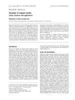
is a fuzzy number (see Figure 1.1).
Example 1.1.2. The fuzzy set represented in Figure 1.2 is not a fuzzy number since
it is not fuzzy convex.
Remark 1.1.1. Any real number is also a fuzzy number,
{
}
R = χ{x} |x is a real number
that means, R ⊂ E .
Here, χ{x} is said to be a singleton fuzzy number for any given real number x ∈ R and
it can be identified with x ∈ R (see Figure 1.3).
Also, fuzzy numbers generalize closed intervals. Indeed, if I denotes the set of all real
4

Figure 1.1: Example of a fuzzy number and its level sets.

interval, then I ∈ E, where
{
}
I = χ[a,b] | [a,b] is real interval ;
Example of a closed interval represented in Figure 1.4 is a fuzzy number.

1.2. Characterization of fuzzy numbers
Definition 1.2.1. [1, 3] For 0 < α ≤ 1, we denote
[u]α = {x ∈ R | u(x) ≥ α} ,
[u]0 = cl {x ∈ R | u(x) > 0} .
Then, [u]α is called the α-level sets of the fuzzy number u. The 1-level set is
called the core of the fuzzy number, while the 0-level set is called the support of the
fuzzy number.
Theorem 1.2.1 (Stacking theorem, [1]). Let u ∈ E be a fuzzy number whose α - level
sets is given by [u]α for all α ∈ [0, 1]. Then
+
−
+
(i) [u]α is a closed interval of the form [u]α = [u−
α , uα ], where uα = inf uα , uα = sup uα
for each α ∈ [0, 1];

(ii) If 0 ≤ α1 ≤ α2 ≤ 1 then uα2 ⊆ uα1 ;
(iii) For any sequence {αn } which converges from below to r ∈ [0, 1], we have
∞
∩

uαn = uα ;

n=1

5


Figure 1.2: Example of a fuzzy set that is not a fuzzy number.

(iv) For any sequence {αn } which converges from above to 0, we have
∪
cl ( ∞
n=1 uαn ) = u0 .
Theorem 1.2.2 (Negoita-Ralescu characterization theorem, Negoita-Ralescu, [1]). Let
{Mα | α ∈ [0, 1]} be a family of subsets that satisfies following conditions:
(i) Mα is a non-empty closed interval for each α ∈ [0, 1];
(ii) If 0 ≤ α1 ≤ α2 ≤ 1 then Mα2 ⊆ Mα1 ;
(iii) For any sequence {αn } which converges from below to α ∈ [0, 1], we have
∩∞
n=1

Mαn = Mα ;

(iv) For any sequence {αn } which converges from above to 0, we have
∪
cl ( ∞
n=1 Mαn ) = M0 .
Then, there exists a unique u ∈ E such that [u]α = Mα for any α ∈ [0, 1].

1.2.1. Some types of fuzzy numbers

The so-called L-R fuzzy numbers are considered as an important fuzzy number
in the theory of fuzzy sets. L-R fuzzy numbers, and their particular cases, as e.g.,
triangular and trapezoidal fuzzy numbers, are very useful in applications.

6


Figure 1.3: A singleton fuzzy number.

Definition 1.2.2. Let L, R : [0, 1] → [0, 1] be two continuous, increasing functions
−
+
+
satisfying L(0) = R(0) = 0, L(1) = R(1) = 1 and a−
0 ≤ a1 ≤ a1 ≤ a0 be real
functions. The fuzzy set u: R → [0, 1] is said to be an L-R fuzzy number if


0
if x < a−

0

)
(

−

x−a
−

L − 0−

if a0 ≤ x < a−
1

a1 −a0

+
(1.1)
u(x) = 1
if a−
1 ≤ x < a1
)
(

+

a0 −x

+

if a+
R a+ −a+

1 ≤ x < a0

0
1



0
if a+
0 ≤ x.
A trapezoidal fuzzy number u can be represented by the quadruple (a, b, c, d)
where a ≤ b ≤ c ≤ d, the functions L and R are linear (see Figure 1.5).


0
if t < a




t−a


 b−a if a ≤ t < b
u(t) =

if b ≤ t ≤ c

1



d−t


d−c




0

if c < t ≤ d
if d < t.

In this case, the endpoints of the α-level set are given by
u−
α = a + α(b − a),
u+
α = d − α(d − c).
7

(1.2)


Figure 1.4: Example of a closed interval interpreted as a fuzzy number.

If we have b = c then the fuzzy number u is called a triangular fuzzy number. Then
a triplet (a, b, c) ∈ R3 , a ≤ b ≤ c is sufficient to represent the triangular fuzzy number
(see Figure 1.6).
+
Example 1.2.1. Let L and R :[0, 1] → [0, 1] given by L(x) = R(x) = x2 , a−
1 = a1 = 1
and a+ = 1, a− = 2, respectively.
Then, the L−R fuzzy number determined by Definition 1.2.2 has the α-level
√
√
α

sets u = [ α, 3 − 2 α] and the shape depicted in Figure 1.7.

A Gaussian fuzzy number has


0


x−x


e− 2σl21
u(x) =
x−x1
−

2
2σr

e




0

the membership degree given by
if x < x1 − aτ1
if x1 − aτl ≤ x < x1
if x1 ≤ x < x1 + aτr

if x + aτr ≤ x,

where x1 is the core of the fuzzy number, σl , σr are the left and right spreads and a > 0
is a tolerance value.
An exponential fuzzy number has the membership degree given by


0
if x < x1 − aτ1




1
e x−x
τl
if x1 − aτl ≤ x < x1
u(x) =
(1.3)
x1 −x

τr
e
if
x
≤
x
<
x
+

aτ

1
1
r



0
if x1 + aτr ≤ x,
where x1 is the core of the exponential fuzzy number τl , τr are the left and right spread
8


Figure 1.5: Example of a trapezoidal fuzzy number

of it respectively, and a represents a tolerance value. Its graph is shown in Figure 1.8

1.2.2. Zadeh’s Extension Principle
Definition 1.2.3. [1] Let a function f : X → Y , where X and Y are crisp sets. Then,
it can be extended to a function F : F(X) → F(Y ) (a fuzzy-valued function) such
that v = F (u), where
{
sup{u(x) : x ∈ X, f (x) = y}, when f −1 (y) ̸= ∅
v(y) =
0,
otherwise,
Then, F is called Zadeh’s extension of f .
Theorem 1.2.3. [1] Let f : X → R be a continuous real-valued function. Then, it
can be extended to a fuzzy-valued function

F :E→E
u → F (u) = v,
where v is a fuzzy number whose level sets [v]α = [vα− , vα+ ] is defined as follows
vα− = inf {f (x) | x ∈ [u]α } ,

α ∈ [0, 1],

vα+ = sup {f (x) | x ∈ [u]α } .

1.2.3. The Sum and Scalar Multiplication
For u, v ∈ E and λ ∈ R, based on the Zadeh’s extension principle, one can
define the sum of two fuzzy numbers u + v and the scalar multiplication λu via their
9


Figure 1.6: Example of a triangular fuzzy number.

level set wises.
[u + v]α = {x + y | x ∈ [u]α , y ∈ [v]α } = [u]α + [v]α ,
(λ · u)α = {λx | x ∈ [u]α } = λ[u]α ,

∀α ∈ [0, 1],

where [u]α +[v]α is the sum of two intervals (as subsets of R) and λ[u]α is the product of
a number and a subset of R. So, fuzzy arithmetic is extended from interval arithmetic.
Example 1.2.2. Let u = (1, 2, 3) and v = (2, 3, 5) be triangular fuzzy numbers with
respective level sets
[u]α = [1 + α, 3 − α],
[v]α = [2 + α, 5 − 2α],
for all α ∈ [0, 1]. Then, sum of u and v is an element w which can be represented in

following parametric form
[w]α = [u]α + [v]α = [3 + 2α, 8 − 3α].
As a consequence of Theorem 1.2.2, we immediately obtain w = (3, 5, 8).
By similar arguments, we can see that the fuzzy number z = (2, 4, 6) is the result
obtained by multiplying the fuzzy number u by 2.
The following theorem deals with the algebraic properties of E .
Theorem 1.2.4. (i) The addition in the space of fuzzy numbers is associative and
commutative i.e.,
u + v = v + u,
10


Figure 1.7: Example of an L-R fuzzy number.

and
u + (v + w) = (u + v) + w,
for all u, v, w ∈ E.
(ii) The fuzzy set ˆ0 = χ{0} ∈ E is the neutral element w.r.t. the addition i.e.,
u + ˆ0 = ˆ0 + u = u,
for any u ∈ E.
(iii) None of u ∈ E \ {R} has an opposite in E (w.r.t. the addition).
(iv) For any a, b ∈ R+ with ab ≥ 0 and any u ∈ E, we have
(a + b) · u = (a · u) + (b · u).
In general, if a, b ∈ R then this property does not hold.
(v) For any λ ∈ R and u, v ∈ E , we have
λ · (u + v) = λ · u + λ · v.
(vi) For any λ, µ ∈ R and any u ∈ E, we have
(λ · µ) · u = λ · (µ · u).

11

Figure 1.8: Example of an exponential fuzzy number.

1.2.4. The product of fuzzy numbers
The product w = u · v of fuzzy numbers u and v, is defined based on Zadeh’s
extension principle. Denote
wα− = inf {x · y | x ∈ [u]α , y ∈ [v]α } ,
wα+ = sup {x · y | x ∈ [u]α , y ∈ [v]α } .
The product attains its extrema at the corners of its domain. Then,
{ − + − − + − + +}
(u · v)−
α = min uα vα , uα vα , uα vα , uα vα ,
and
{ − + − − + − + +}
(u · v)+
α = max uα vα , uα vα , uα vα , uα vα .
Example 1.2.3. Let u = (1, 2, 3) and v = (2, 3, 5). Then,
(u · v)−
α = (1 + α)(2 + α)
(u · v)+
α = (3 − α)(5 − 2α),
where (u · v)1 = [6, 6] , (u · v)0 = [2, 15].
Theorem 1.2.5. (i) The singleton fuzzy set ˆ1 = χ{1} ∈ E is the neutral element w.r.t.
the multiplication i.e., u · ˆ1 = ˆ1 · u = u, for any u ∈ E.
(ii) None of u ∈ E \ R has an inverse in E(w.r.t. the multiplication).
(iii) For any u, v, w ∈ E we have
((u + v) · w)λ ⊆ (u · w)λ + (v · w)λ, for all λ ∈ R.
In general, the distribution property does not hold.
12

(iv) For any u, v, w ∈ E such that none of their supports contains 0, we have
u · (v · w) = (u · v) · w.
Proposition 1.2.6. If u and v are positive fuzzy numbers then the fuzzy number w,
defined by w = u · v, has the level sets [w]α = [wα− , wα+ ], where
−
− −
− −
wα− = u−
α v1 + u1 vα − u1 v1 ,

and
+
+ +
+ +
wα+ = u+
α v1 + u1 vα − u1 v1 ,

for every α ∈ [0, 1]. Moreover, w is a positive fuzzy number.

1.2.5. The difference of fuzzy numbers
Definition 1.2.4. [3, 4] The Hukuhara difference (H-difference ) of two fuzzy number
u and v is defined by
u ⊖H v = w ⇔ u = v + w,
where + represents for the standard fuzzy addition.
If u ⊖H v exists, its α − cuts are
−
+
+

[u ⊖H v]α = [u−
α − vα , uα − vα ].

We see that u ⊖H u = ˆ0 for any fuzzy numbers u, but as we have earlier discussed
u − u ̸= ˆ0.
Example 1.2.4. Let u = [0, 1], −u = [−1, 0] then
u − u = u + (−u) ̸= ˆ0 = [0, 0].
Definition 1.2.5. [3, 4] Let u, v ∈ E. Then, the generalized Hukuhara difference
(gH-difference for short) is the fuzzy number w, if it exists, such that
{
(i) u = v + w, or
u ⊖gH v = w ⇔
(ii) v = u + (−w)
Proposition 1.2.7. For any u, v ∈ E, we have
[
{
}
{ −
}]
−
+
+
−
+
+
[u ⊖gH v]α = min u−
−
v
,
u

−
v
,
max
u
−
v
,
u
−
v
.
α
α
α
α
α
α
r
α
Example 1.2.5. Let u = (1, 2, 3) and v = (2, 3, 5) be positive triangular fuzzy numbers.
Then, the α− cuts of u and v are given by
[u]α = [1 + α, 3 − α],
[v]α = [2 + α, 5 − 2α],
respectively. Then, according to Proposition 1.2.7, we can see that
[u ⊖gH v]α = [min {−1, −2 + α} , max {−1, −2 + α}] = [−2, −1].
13


1.3. Fuzzy derivative and integral

Theorem 1.3.1. [1] Let f : (a, b) ⊆ R → E be a fuzzy function and x0 ∈ (a, b). Then,
f (x) is strongly generalized Hukuhara differentiable (SGH-differentiable) at the point
x0 , in the first form, if there exists an element fSGH (x0 ) ∈ E such that for h > 0
sufficiently near zero, f (x0 + h) ⊖H f (x0 ),f (x0 ) ⊖H f (x0 − h) exist and the limits
lim

h→0

f (x0 + h) ⊖H f (x0 )
f (x0 ) ⊖H f (x0 − h)
′
= lim
= fSGH (x0 )
h→0
h
h

holds. f (x) is strongly generalized Hukuhara differentiable (SGH-differentiable) at the
′
point x0 , in the second form, if there exists an element fSGH (x0 ) ∈ E1 such that for h
> 0 sufficiently near zero, there f (x0 ) ⊖H f (x0 + h), f (x0 − h) ⊖H f (x0 ) and the limits
f (x0 ) ⊖H f (x0 + h)
f (x0 − h) ⊖H f (x0 )
′
= lim
= fSGH (x0 ) .
h→0
h→0
−h
−h

lim

Definition 1.3.1. [2, 3] Let f : (a, b) ⊆ R → E be a fuzzy function and x0 ∈ (a, b).
Then, f (x) is generalized Hukuhara differentiable (gH-differentiable) at the point x0 , if
′
there exists an element fgH (x) ∈ E such that for h sufficiently near zero the following
limit exists
f (x0 + h) ⊖gH f (x0 )
′
= fgH (x0 ).
h→0
h
lim

Theorem 1.3.2. [2] Let f : (a, b) ⊆ R → E be a function such that [f (x)]α =
[fα− (x), fα+ (x)], x ∈ [0, 1]. Suppose that the real-valued functions fα− (x), fα+ (x) are
differentiable for all α ∈ [0, 1]. Then, the fuzzy-valued function f (x) is gH-differentiable
at a fix x ∈ (a, b) if and only if one of the following two cases holds:
−
+
1) fα− (x) and fα+ (x) are increasing and decreasing functions of α, fα=1
(x) ≤ fα=1
(x).
−
−
(x) ≤ fα=1
2) fα− (x) and fα+ (x) are increasing and decreasing functions of α, fα=1
(x).

Futhermore,

[
{
}
{ ′ −
}]
′
′ +
′ +
[fgH
(x)]α = min (f ′ )−
.
α (x), (f )α (x) , max (f )α (x), (f )α (x)
The definition of Lebesgue integral for fuzzy-valued functions [1] is in the sense
of Aumann integral for set-valued functions [5].
Definition 1.3.2. [2, 3] Assume that f : [a, b] → E is a fuzzy-valued function with
parametric form [f (t)]α = [fα− (t), fα+ (t)] for all t ∈ [a, b], α ∈ [0, 1] and fα− (t), fα+ (t)
are measurable and Lebesgue integrable on [a, b]. Then the Lebesgue integral of f is
∫b
denoted by a f (t)dt, which can be written in following parametric form
[∫ b
]α [∫ b
]
∫ b
+
−
fα (t)dt for all α ∈ [0, 1].
f (t)dt =
fα (t)dt,
a

a

a

1

Denote L ([a, b], E) by the space of all Lebesgue integrable fuzzy-valued functions on [a, b]. The properties of integrable fuzzy-valued function used throughout this
thesis can be referred from [1].
14


Chapter 2
Granular differentiability of fuzzy-valued functions

2.1. Granular representation
Definition 2.1.1. [4] For a fuzzy number u : [a, b] → [0, 1] with parametric form
+
gr
[u]α = [u−
: [0, 1] × [0, 1] → [a, b]
α , uα ], the horizontal membership function (HMF) u
gr
−
+
−
with x = u (α, αu ) = uα + (uα − uα )αu in which “gr” stands for the granule of
information included in x ∈ [a, b], α ∈ [0, 1] is the membership degree of x in u(x) ,
αu ∈ [0, 1] is called relative-distance-measure (RDM).
Remark 2.1.1. We can also denote the HMF of u ∈ E by H(u)
ugr (α, αu ). In

particular, if u = (a, b, c) is a triangular fuzzy number and v = (a, b, c, d) is a trapezoidal
fuzzy number then the HMF of u and v are H(u) = a + (b − a)α + (1 − α)(c − a)αu ,
H(v) = a + (b − a)α + [(d − a) − (d − a + b − c)α]αv in which α, αu , αv ∈ [0, 1].
Example 2.1.1. Let v = (2, 4, 6, 9) then H(u) = 2α + [9 − 13α]αv (see Figure 2.1).

Figure 2.1: The trapezoidal fuzzy interval number u = (2, 4, 6, 9).

Proposition 2.1.1. [4] The α−level sets of u ∈ E which are the span of the information granule can be obtained by using
[
]
gr
gr
−1 gr
α
H (u (α, αu )) = [u] = inf min u (β, αu ), sup max u (β, αu ) ,
(2.1)
β≥α αu

in which α, αu ∈ [0, 1].
15

β≥α αu


Definition 2.1.2. Let u, v ∈ E with the presentation HMF respectively,
+
−
ugr (α, αu ) = u−
α + (uα − uα )αu ,

v gr (α, αv ) = vα− + (vα+ − vα− )αv ,
for all α, αu , αv ∈ [0, 1]. Then, we say that
(i) u = v if ugr (α, αu ) = v gr (α, αv ) (or H(u) = H(v)) for all αu = αv ∈ [0, 1].
(ii) u ≤ v if ugr (α, αu ) ≤ v gr (α, αv ) ( or H(u) ≤ H(v)) for all αu = αv ∈ [0, 1].

2.2. Granular operations
Definition 2.2.1. [4] Denote by “⊙” the one of the four operators in E: the addition,
the subtraction, the multiplication or division operator. Then H(u ⊙ v) H(u) ∗ H(v)
where denote “*” is one of the four operators in R. It should be noted that 0 ̸=
v gr (α, αv ) when “⊙” denotes the division operator. And the difference in this sense is
called granular difference (gr-difference), denoted by ⊖gr .
Proposition 2.2.1. [4] Let m = u⊙v then [m]α = H−1 (ugr (α, αu )⊙v gr (α, αv )) always
presents α-level sets of fuzzy number m.
Definition 2.2.2. If f : [a, b] → E is a fuzzy-valued function including n distinct fuzzy
numbers u1 , u2 , ..., un . The HMF H(f (t)) f gr (t, α, αf ) of f (t) is defined as
f gr : [a, b] × [0, 1] × [0, 1]n → [c, d] ⊆ R,
where αf

(αu1 , αu2 , ..., αun ).

Example 2.2.1. Let u = (1, 2, 3) and v = (−5, −3, −1) with respective HMFs ugr (α, αu ) =
1 + α + 2(1 − α)αu and v gr (α, αv ) = −5 + 2α + 4(1 − α)αv for α, αu , αv ∈ [0, 1].
Consider fuzzy-valued function f (t) = e2t u + tv with t ∈ [−2, 2]. The HMF of
function f is given as follows
H(f (t)) = f gr (t, α, αu , αv )
= (1 + α)e2t + (2α − 5)t + 2(1 − α)e2t αu + 4t(1 − α)αv ,
The graphical representation of f is shown in Figure 2.2.

2.3. The granular metric space (E, Dgr )
Definition 2.3.1. [4] The granular distance between u and v in E is the function

Dgr : E × E → [0, ∞) given by
Dgr (u, v) = sup max |ugr (α, αu ) − v gr (α, αv )|.
α

αu ,αv

It is easy to see that Dgr is a metric on the space E.

16

(2.2)


Figure 2.2: The curves of α -level sets of f (t) = e2t u + tv in Example 2.2.1 in which the blue and red
curves correspond to left and right end-points functions at any α-level sets and the black curve stands
for the level α = 1.

Proof. For all u, v ∈ E whose granular representations are ugr (α, αu ) , v gr (α, αv ),
we have:
|ugr (α, αu ) − v gr (α, αv )| ≥ 0,
for all α, αu , αv ∈ [0, 1]. Hence,
Dgr (u, v) = sup max |ugr (α, αu ) − v gr (α, αv )| ≥ 0.
α

αu ,αv

In addition, for all α ∈ [0, 1], we can see that
Dgr (u, v) = 0 ⇔ sup max |ugr (α, αu ) − v gr (α, αv )| = 0
α

αu ,αv

⇔ max |ugr (α, αu ) − v gr (α, αv )| = 0
αu ,αv

⇔ |ugr (α, αu ) − v gr (α, αv )| = 0
⇔ ugr (α, αu ) = v gr (α, αv ).
for all α, αu , αv ∈ [0, 1], Thus, according to Definition 2.2.2, we have that u = v.
We also have
Dgr (u, v) = sup max |ugr (α, αu ) − v gr (α, αv )|
α

αu ,αv

17


= sup max |v gr (α, αv ) − ugr (α, αu )|
α αu ,αv
gr

= D (v, u).
Due to the fact that
|ugr (α, αu ) − v gr (α, αv )| = |ugr (α, αu ) − wgr (α, αw ) + wgr (α, αw ) − v gr (α, αv )|
≤ |ugr (α, αu ) − wgr (α, αw )| + |wgr (α, αw ) − v gr (α, αv )|,
which follows
|ugr (α, αu ) − v gr (α, αv )| ≤ max {|ugr (α, αu ) − wgr (α, αw )| + |wgr (α, αw ) − v gr (α, αv )|}
αw ,αv

⇒ max |ugr (α, αu ) − v gr (α, αv )| ≤ max {|ugr (α, αu ) − wgr (α, αw )|

αu ,αv

αw ,αv

+|wgr (α, αw ) − v gr (α, αv )|}
⇒ max |ugr (α, αu ) − v gr (α, αv )| ≤ sup max {|ugr (α, αu ) − wgr (α, αw )|
αu ,αv

α

αw ,αv

+|wgr (α, αw ) − v gr (α, αv )|}
⇒ sup max |ugr (α, αu ) − v gr (α, αv )| ≤ sup max {|ugr (α, αu ) − wgr (α, αw )|
α

αu ,αv

α

αw ,αv

+|wgr (α, αw ) − v gr (α, αv )|} ,
for all α, αu , αw αv ∈ [0, 1], that means
Dgr (u, v) ≤ Dgr (u, w) + Dgr (w, v).
Thus, Dgr is a metric on the space E.
Proposition 2.3.1. The space E endowed with granular metric Dgr is a complete
metric space.
Proof. If any Cauchy sequence of fuzzy numbers by Dgr is convergent in E, then the
proof is completed. Suppose un ∈ E; n ≥ 1 is a Cauchy sequence. Then,

∀ϵ > 0, ∃N ≥ 1 ∋ Dgr (un , un+p < ϵ), ∀n ≥ N, p ≥ 1,
which means
sup
α

max

αun ,αun+p

gr
| ugr
n (α, αun ) − un+p (α, αun+p ) < ϵ | ;

or equivalently
gr
| ugr
n (α, αun ) − un+p (α, αun+p ) < ϵ | .

Therefore, ugr (α, αun ) is a Cauchy sequence in the space of the real numbers. Then,
ugr (α, αun ) is convergent in R.
+
−
Based on Definition 2.1.1,we get ugr
n (α, αun ) = (1 − αun )(un )α + (αun )α (un ). Since
+
−
ugr
n (α, αun ) is convergent and 0 ≤ αun ≤ 1, the sequences (un )α , (un )α are convergent.
−
+

+
−
Suppose lim (un )−
α = (un )α , and lim (un )α = (un )α . Due to the fact that (un )α ≤
n→∞

n→∞

−
+
(un )+
α , we will have uα ≤ uα . For completing the proof, we need to show that the
+
interval [u−
α , uα ] is the α-level set of a fuzzy number, and hence it is omitted.

18


Figure 2.3: The gr-distance between two fuzzy numbers u = (0, 1, 2) and v = (3, 6, 7, 9).

Example 2.3.1.
a. Let u = (0, 1, 2) and v = (3, 6, 7, 9) be triangular and trapezoidal fuzzy numbers,
respectively (see Figure 2.3). Then, from the formula (2.2), it follows that the
distance between two fuzzy numbers u = (0, 1, 2) and v = (3, 6, 7, 9) is given by
Dgr (u, v) = sup max |ugr (α, αu ) − v gr (α, αv )|
α

αu ,αv

= sup max |3 + 2α + (6 − 5α)αv − (2 − 2α)αu |
α

αu ,αv

= sup |9 − 3α| = 9.
α

where ugr (α, αu ) = α + (2 − 2α)αu , v gr (α, αv ) = 3 + 3α + (6 − 5α)αv for α, αu ,
αv ∈ [0, 1].
b. Let u = (4, 8, 10) and v = (1, 5, 7) be triangular fuzzy numbers with HMFs
ugr (α, αu ) = 4(1 + α) + 6(1 − α)αu and v gr (α, αv ) = 1 + 4α + 6(1 − α)αv , for
α, αu , αv ∈ [0, 1]. Then, as a result of formula (2.2), the distance between u and
v is given by
Dgr (u, v) = sup max |ugr (α, αu ) − v gr (α, αv )|
α

αu ,αv

= sup max |3 + 6(1 − α)(αu − αv )|
α

αu ,αv

= sup |9 − 6α| = 9.
α

c. Let u = (1, 2, 4) and v = (0, 1, 4, 5) be triangular and trapezoidal fuzzy numbers
with respective HMFs ugr (α, αu ) = 1 + α + 3(1 − α)αu and v gr (α, αv ) = α + (5 −
2α)αv , for α, αu , αv ∈ [0, 1] (see Figure 2.4). Then, the gr-distance of u and v can

be computed as follows
Dgr (u, v) = sup max |ugr (α, αu ) − v gr (α, αv )|
α

αu ,αv

= sup max |1 + 3(1 − α)αu − (5 − 2α)αv )|
α

αu ,αv

19


Figure 2.4: The gr-distance between two fuzzy numbers u = (1, 2, 4) and v = (0, 1, 4, 5).

= sup |4 − 3α| = 4.
α

Definition 2.3.2. Let f : [a, b] ⊂ R → E and t0 ∈ [a, b]. Then, we say that the
function f has the finite limit as t tends to t0 if and only if there exists τ ∈ E such that
lim Dgr (f (t), τ ) = 0, that is ∀ ϵ > 0, ∃ δ(t0 , ϵ) > 0 such that ∀t ∈ [a, b] : 0 < |t−t0 | < δ,

t→t0

it implies Dgr (f (t), τ ) < ϵ.
Definition 2.3.3. (The continuity) A fuzzy-valued function f : (a, b) ⊂ R → E is said
to be continuous on (a, b) if for each t0 ∈ (a, b), for all ϵ > 0, there exists δ > 0 such
that ∀t ∈ (a, b) : |t − t0 | < δ, Dgr (f (t), f (t0 )) < ϵ, i.e., lim Dgr (f (t), f (t0 )) = 0.
t→t0

Lemma 2.3.2. Let u, v, e ∈ E and λ ∈ R. Then, the following statements hold
(i) Dgr (u + e, v + e) = Dgr (u, v).
(ii) Dgr (λu, λv) = |λ|Dgr (u, v).
Proof. (i) By the formula (2.2), we have
Dgr (u + e, v + e) = sup max |[ugr (α, αu ) + egr (α, αe )] − [v gr (α, αv ) + egr (α, αe )]|
α

αu ,αv ,αe

= sup max |ugr (α, αu ) − v gr (α, αv )|
α αu ,αv
gr

= D (u, v).
(ii) Similarly, we also have
Dgr (λu, λv) = sup max |λugr (α, αu ) − λv gr (α, αv )|
α

αu ,αv

= |λ| sup max |ugr (α, αu ) − v gr (α, αv )|
α αu ,αv
gr

= |λ|D (u, v).
Hence, the proof is complete.

20