Statistical tools for program evaluation methods and applications to economic policy, public health, and education
Bạn đang xem bản rút gọn của tài liệu. Xem và tải ngay bản đầy đủ của tài liệu tại đây (39.33 MB, 530 trang )
Jean-Michel Josselin
Benoît Le Maux
Statistical Tools
for Program
Evaluation
Methods and Applications to Economic
Policy, Public Health, and Education
Statistical Tools for Program Evaluation
Jean-Michel Josselin • Benoıˆt Le Maux
Statistical Tools for
Program Evaluation
Methods and Applications to Economic
Policy, Public Health, and Education
Jean-Michel Josselin
Faculty of Economics
University of Rennes 1
Rennes, France
Benoıˆt Le Maux
Faculty of Economics
University of Rennes 1
Rennes, France
ISBN 978-3-319-52826-7
ISBN 978-3-319-52827-4
DOI 10.1007/978-3-319-52827-4
(eBook)
Library of Congress Control Number: 2017940041
# Springer International Publishing AG 2017
This work is subject to copyright. All rights are reserved by the Publisher, whether the whole or part of
the material is concerned, specifically the rights of translation, reprinting, reuse of illustrations,
recitation, broadcasting, reproduction on microfilms or in any other physical way, and transmission
or information storage and retrieval, electronic adaptation, computer software, or by similar or
dissimilar methodology now known or hereafter developed.
The use of general descriptive names, registered names, trademarks, service marks, etc. in this
publication does not imply, even in the absence of a specific statement, that such names are exempt
from the relevant protective laws and regulations and therefore free for general use.
The publisher, the authors and the editors are safe to assume that the advice and information in this
book are believed to be true and accurate at the date of publication. Neither the publisher nor the
authors or the editors give a warranty, express or implied, with respect to the material contained
herein or for any errors or omissions that may have been made. The publisher remains neutral with
regard to jurisdictional claims in published maps and institutional affiliations.
Printed on acid-free paper
This Springer imprint is published by Springer Nature
The registered company is Springer International Publishing AG
The registered company address is: Gewerbestrasse 11, 6330 Cham, Switzerland
Acknowledgments
We would like to express our gratitude to those who helped us and made the
completion of this book possible.
First of all, we are deeply indebted to the Springer editorial team and particularly
Martina BIHN whose support and encouragement allowed us to finalize this
project.
Furthermore, we have benefited from helpful comments by colleagues and we
would like to acknowledge the help of Maurice BASLE´, Arthur CHARPENTIER,
Pauline CHAUVIN, Salah GHABRI, and Christophe TAVE´RA. Of course, any
mistake that may remain is our entire responsibility.
In addition, we are grateful to our students who have been testing and
experimenting our lectures for so many years. Parts of the material provided here
have been taught at the Bachelor and Master levels, in France and abroad. Several
students and former students have been helping us improve the book. We really
appreciated their efforts and are very grateful to them: Erwan AUTIN, Benoıˆt
´ LOVA
´ , and Adrien VEZIE.
CARRE´, Aude DAILLE`RE, Kristy´na DOSTA
Finally, we would like to express our sincere gratefulness to our families for
their continuous support and encouragement.
v
Contents
1
Statistical Tools for Program Evaluation: Introduction and
Overview . . . . . . . . . . . . . . . . . . . . . . . . . . . . . . . . . . . . . . . . . . . . .
1.1
The Challenge of Program Evaluation . . . . . . . . . . . . . . . . . . .
1.2
Identifying the Context of the Program . . . . . . . . . . . . . . . . . .
1.3
Ex ante Evaluation Methods . . . . . . . . . . . . . . . . . . . . . . . . . .
1.4
Ex post Evaluation . . . . . . . . . . . . . . . . . . . . . . . . . . . . . . . . .
1.5
How to Use the Book? . . . . . . . . . . . . . . . . . . . . . . . . . . . . . .
Bibliography . . . . . . . . . . . . . . . . . . . . . . . . . . . . . . . . . . . . . . . . . .
Part I
1
1
4
6
9
11
12
Identifying the Context of the Program
2
Sampling and Construction of Variables . . . . . . . . . . . . . . . . . . . . .
2.1
A Step Not to Be Taken Lightly . . . . . . . . . . . . . . . . . . . . . . .
2.2
Choice of Sample . . . . . . . . . . . . . . . . . . . . . . . . . . . . . . . . . .
2.3
Conception of the Questionnaire . . . . . . . . . . . . . . . . . . . . . . .
2.4
Data Collection . . . . . . . . . . . . . . . . . . . . . . . . . . . . . . . . . . .
2.5
Coding of Variables . . . . . . . . . . . . . . . . . . . . . . . . . . . . . . . .
Bibliography . . . . . . . . . . . . . . . . . . . . . . . . . . . . . . . . . . . . . . . . . .
15
15
16
22
27
33
43
3
Descriptive Statistics and Interval Estimation . . . . . . . . . . . . . . . .
3.1
Types of Variables and Methods . . . . . . . . . . . . . . . . . . . . . .
3.2
Tabular Displays . . . . . . . . . . . . . . . . . . . . . . . . . . . . . . . . .
3.3
Graphical Representations . . . . . . . . . . . . . . . . . . . . . . . . . . .
3.4
Measures of Central Tendency and Variability . . . . . . . . . . . .
3.5
Describing the Shape of Distributions . . . . . . . . . . . . . . . . . .
3.6
Computing Confidence Intervals . . . . . . . . . . . . . . . . . . . . . .
References . . . . . . . . . . . . . . . . . . . . . . . . . . . . . . . . . . . . . . . . . . .
.
.
.
.
.
.
.
.
45
45
47
54
64
69
77
87
4
Measuring and Visualizing Associations . . . . . . . . . . . . . . . . . . . .
4.1
Identifying Relationships Between Variables . . . . . . . . . . . . .
4.2
Testing for Correlation . . . . . . . . . . . . . . . . . . . . . . . . . . . . .
4.3
Chi-Square Test of Independence . . . . . . . . . . . . . . . . . . . . .
.
.
.
.
89
89
92
99
vii
viii
Contents
4.4
Tests of Difference Between Means . . . . . . . . . . . . . . . . . . . . .
4.5
Principal Component Analysis . . . . . . . . . . . . . . . . . . . . . . . . .
4.6
Multiple Correspondence Analysis . . . . . . . . . . . . . . . . . . . . . .
References . . . . . . . . . . . . . . . . . . . . . . . . . . . . . . . . . . . . . . . . . . . .
105
113
126
135
5
Econometric Analysis . . . . . . . . . . . . . . . . . . . . . . . . . . . . . . . . . .
5.1
Understanding the Basic Regression Model . . . . . . . . . . . . . .
5.2
Multiple Regression Analysis . . . . . . . . . . . . . . . . . . . . . . . .
5.3
Assumptions Underlying the Method of OLS . . . . . . . . . . . . .
5.4
Choice of Relevant Variables . . . . . . . . . . . . . . . . . . . . . . . .
5.5
Functional Forms of Regression Models . . . . . . . . . . . . . . . .
5.6
Detection and Correction of Estimation Biases . . . . . . . . . . . .
5.7
Model Selection and Analysis of Regression Results . . . . . . .
5.8
Models for Binary Outcomes . . . . . . . . . . . . . . . . . . . . . . . . .
References . . . . . . . . . . . . . . . . . . . . . . . . . . . . . . . . . . . . . . . . . . .
.
.
.
.
.
.
.
.
.
.
137
137
147
153
156
164
167
174
180
187
6
Estimation of Welfare Changes . . . . . . . . . . . . . . . . . . . . . . . . . . .
6.1
Valuing the Consequences of a Project . . . . . . . . . . . . . . . . .
6.2
Contingent Valuation . . . . . . . . . . . . . . . . . . . . . . . . . . . . . .
6.3
Discrete Choice Experiment . . . . . . . . . . . . . . . . . . . . . . . . .
6.4
Hedonic Pricing . . . . . . . . . . . . . . . . . . . . . . . . . . . . . . . . . .
6.5
Travel Cost Method . . . . . . . . . . . . . . . . . . . . . . . . . . . . . . .
6.6
Health-Related Quality of Life . . . . . . . . . . . . . . . . . . . . . . .
References . . . . . . . . . . . . . . . . . . . . . . . . . . . . . . . . . . . . . . . . . . .
.
.
.
.
.
.
.
.
189
189
191
200
211
216
221
230
Part II
Ex ante Evaluation
7
Financial Appraisal . . . . . . . . . . . . . . . . . . . . . . . . . . . . . . . . . . . .
7.1
Methodology of Financial Appraisal . . . . . . . . . . . . . . . . . . .
7.2
Time Value of Money . . . . . . . . . . . . . . . . . . . . . . . . . . . . . .
7.3
Cash Flows and Sustainability . . . . . . . . . . . . . . . . . . . . . . . .
7.4
Profitability Analysis . . . . . . . . . . . . . . . . . . . . . . . . . . . . . .
7.5
Real Versus Nominal Values . . . . . . . . . . . . . . . . . . . . . . . . .
7.6
Ranking Investment Strategies . . . . . . . . . . . . . . . . . . . . . . . .
7.7
Sensitivity Analysis . . . . . . . . . . . . . . . . . . . . . . . . . . . . . . .
References . . . . . . . . . . . . . . . . . . . . . . . . . . . . . . . . . . . . . . . . . . .
.
.
.
.
.
.
.
.
.
235
235
238
244
249
255
257
263
266
8
Budget Impact Analysis . . . . . . . . . . . . . . . . . . . . . . . . . . . . . . . . .
8.1
Introducing a New Intervention Amongst Existing Ones . . . . . .
8.2
Analytical Framework . . . . . . . . . . . . . . . . . . . . . . . . . . . . . . .
8.3
Budget Impact in a Multiple-Supply Setting . . . . . . . . . . . . . . .
8.4
Example . . . . . . . . . . . . . . . . . . . . . . . . . . . . . . . . . . . . . . . . .
8.5
Sensitivity Analysis with Visual Basic . . . . . . . . . . . . . . . . . . .
References . . . . . . . . . . . . . . . . . . . . . . . . . . . . . . . . . . . . . . . . . . . .
269
269
271
275
277
281
288
Contents
ix
9
Cost Benefit Analysis . . . . . . . . . . . . . . . . . . . . . . . . . . . . . . . . . . .
9.1
Rationale for Cost Benefit Analysis . . . . . . . . . . . . . . . . . . . . .
9.2
Conceptual Foundations . . . . . . . . . . . . . . . . . . . . . . . . . . . . .
9.3
Discount of Benefits and Costs . . . . . . . . . . . . . . . . . . . . . . . .
9.4
Accounting for Market Distortions . . . . . . . . . . . . . . . . . . . . . .
9.5
Deterministic Sensitivity Analysis . . . . . . . . . . . . . . . . . . . . . .
9.6
Probabilistic Sensitivity Analysis . . . . . . . . . . . . . . . . . . . . . . .
9.7
Mean-Variance Analysis . . . . . . . . . . . . . . . . . . . . . . . . . . . . .
Bibliography . . . . . . . . . . . . . . . . . . . . . . . . . . . . . . . . . . . . . . . . . .
291
291
294
299
306
311
313
321
324
10
Cost Effectiveness Analysis . . . . . . . . . . . . . . . . . . . . . . . . . . . . . .
10.1 Appraisal of Projects with Non-monetary Outcomes . . . . . . . .
10.2 Cost Effectiveness Indicators . . . . . . . . . . . . . . . . . . . . . . . . .
10.3 The Efficiency Frontier Approach . . . . . . . . . . . . . . . . . . . . .
10.4 Decision Analytic Modeling . . . . . . . . . . . . . . . . . . . . . . . . .
10.5 Numerical Implementation in R-CRAN . . . . . . . . . . . . . . . . .
10.6 Extension to QALYs . . . . . . . . . . . . . . . . . . . . . . . . . . . . . . .
10.7 Uncertainty and Probabilistic Sensitivity Analysis . . . . . . . . .
10.8 Analyzing Simulation Outputs . . . . . . . . . . . . . . . . . . . . . . . .
References . . . . . . . . . . . . . . . . . . . . . . . . . . . . . . . . . . . . . . . . . . .
.
.
.
.
.
.
.
.
.
.
325
325
328
336
342
351
357
358
371
382
11
Multi-criteria Decision Analysis . . . . . . . . . . . . . . . . . . . . . . . . . .
11.1 Key Concepts and Steps . . . . . . . . . . . . . . . . . . . . . . . . . . . .
11.2 Problem Structuring . . . . . . . . . . . . . . . . . . . . . . . . . . . . . . .
11.3 Assessing Performance Levels with Scoring . . . . . . . . . . . . . .
11.4 Criteria Weighting . . . . . . . . . . . . . . . . . . . . . . . . . . . . . . . .
11.5 Construction of a Composite Indicator . . . . . . . . . . . . . . . . . .
11.6 Non-Compensatory Analysis . . . . . . . . . . . . . . . . . . . . . . . . .
11.7 Examination of Results . . . . . . . . . . . . . . . . . . . . . . . . . . . . .
References . . . . . . . . . . . . . . . . . . . . . . . . . . . . . . . . . . . . . . . . . . .
.
.
.
.
.
.
.
.
.
385
385
388
390
395
398
401
410
416
Part III
12
Ex post Evaluation
Project Follow-Up by Benchmarking . . . . . . . . . . . . . . . . . . . . . .
12.1 Cost Comparisons to a Reference . . . . . . . . . . . . . . . . . . . . .
12.2 Cost Accounting Framework . . . . . . . . . . . . . . . . . . . . . . . . .
12.3 Effects of Demand Structure and Production Structure
on Cost . . . . . . . . . . . . . . . . . . . . . . . . . . . . . . . . . . . . . . . .
12.4 Production Structure Effect: Service-Oriented Approach . . . . .
12.5 Production Structure Effect: Input-Oriented Approach . . . . . .
12.6 Ranking Through Benchmarking . . . . . . . . . . . . . . . . . . . . . .
References . . . . . . . . . . . . . . . . . . . . . . . . . . . . . . . . . . . . . . . . . . .
. 419
. 419
. 423
.
.
.
.
.
426
433
436
440
441
x
13
14
Contents
Randomized Controlled Experiments . . . . . . . . . . . . . . . . . . . . . . .
13.1 From Clinical Trials to Field Experiments . . . . . . . . . . . . . . . .
13.2 Random Allocation of Subjects . . . . . . . . . . . . . . . . . . . . . . . .
13.3 Statistical Significance of a Treatment Effect . . . . . . . . . . . . . .
13.4 Clinical Significance and Statistical Power . . . . . . . . . . . . . . . .
13.5 Sample Size Calculations . . . . . . . . . . . . . . . . . . . . . . . . . . . .
13.6 Indicators of Policy Effects . . . . . . . . . . . . . . . . . . . . . . . . . . .
13.7 Survival Analysis with Censoring: The Kaplan-Meier
Approach . . . . . . . . . . . . . . . . . . . . . . . . . . . . . . . . . . . . . . . .
13.8 Mantel-Haenszel Test for Conditional Independence . . . . . . . . .
References . . . . . . . . . . . . . . . . . . . . . . . . . . . . . . . . . . . . . . . . . . . .
443
443
448
453
463
471
474
Quasi-experiments . . . . . . . . . . . . . . . . . . . . . . . . . . . . . . . . . . . .
14.1 The Rationale for Counterfactual Analysis . . . . . . . . . . . . . . .
14.2 Difference-in-Differences . . . . . . . . . . . . . . . . . . . . . . . . . . .
14.3 Propensity Score Matching . . . . . . . . . . . . . . . . . . . . . . . . . .
14.4 Regression Discontinuity Design . . . . . . . . . . . . . . . . . . . . . .
14.5 Instrumental Variable Estimation . . . . . . . . . . . . . . . . . . . . . .
References . . . . . . . . . . . . . . . . . . . . . . . . . . . . . . . . . . . . . . . . . . .
489
489
492
498
512
519
530
.
.
.
.
.
.
.
480
483
487
1
Statistical Tools for Program Evaluation:
Introduction and Overview
1.1
The Challenge of Program Evaluation
The past 30 years have seen a convergence of management methods and practices
between the public sector and the private sector, not only at the central government
level (in particular in Western countries) but also at upper levels (European
commission, OECD, IMF, World Bank) and local levels (municipalities, cantons,
regions). This “new public management” intends to rationalize public spending,
boost the performance of services, get closer to citizens’ expectations, and contain
deficits. A key feature of this evolution is that program evaluation is nowadays part
of the policy-making process or, at least, on its way of becoming an important step
in the design of public policies. Public programs must show evidence of their
relevance, financial sustainability and operationality. Although not yet systematically enacted, program evaluation intends to grasp the impact of public projects on
citizens, as comprehensively as possible, from economic to social and environmental consequences on individual and collective welfare. As can be deduced, the task
is highly challenging as it is not so easy to put a value on items such as welfare,
health, education or changes in environment. The task is all the more demanding
that a significant level of expertise is required for measuring those impacts or for
comparing different policy options.
The present chapter offers an introduction to the main concepts that will be used
throughout the book. First, we shall start with defining the concept of program
evaluation itself. Although there is no consensus in this respect, we may refer to the
OECD glossary which states that evaluation is the “process whereby the activities
undertaken by ministries and agencies are assessed against a set of objectives or
criteria.” According to Michael Quinn Patton, former President of the American
Evaluation Association, program evaluation can also be defined as “the systematic
collection of information about the activities, characteristics, and outcomes of
programs, for use by people to reduce uncertainties, improve effectiveness, and
make decisions.” We may also propose our own definition of the concept: program
evaluation is a process that consists in collecting, analyzing, and using information
# Springer International Publishing AG 2017
J.-M. Josselin, B. Le Maux, Statistical Tools for Program Evaluation,
DOI 10.1007/978-3-319-52827-4_1
1
2
1
Statistical Tools for Program Evaluation: Introduction and Overview
Efϐiciency
Relevance
Effectiveness
Needs
Design
Inputs
Outputs
Short & long-term outcomes
Indicators of
context
Objectives/target
Indicators of
means
Indicators of
realization
Result and impact indicators
Fig. 1.1 Program evaluation frame
to assess the relevance of a public program, its effectiveness and its efficiency.
Those concepts are further detailed below. Note that a distinction will be made
throughout the book between a program and its alternative and competing strategies
of implementation. By strategies, we mean the range of policy options or public
projects that are considered within the framework of the program. The term
program, on the other hand, has a broader scope and relates to the whole range of
steps that are carried out in order to attain the desired goal.
As shown in Fig. 1.1, a program can be described in terms of needs, design,
inputs and outputs, short and long-term outcomes. Needs can be defined as a desire
to improve current outcomes or to correct them if they do not reach the required
standard. Policy design is about the definition of a course of action intended to meet
the needs. The inputs represent the resources or means (human, financial, and
material) used by the program to carry out its activities. The outputs stand for
what comes out directly from those activities (the intervention) and which are under
direct control of the authority concerned. The short-term and long-term outcomes
stand for effects that are induced by the program but not directly under the control
of the authority. Those include changes in social, economic, environmental and
other indicators.
Broadly speaking, the evaluation process can be represented through a linear
sequence of four phases (Fig. 1.1). First, a context analysis must gather information
and determine needs. For instance, it may evidence a high rate of school dropout
among young people in a given area. A program may help teachers, families and
children and contribute to prevent or contain dropout. If the authority feels that the
consequences on individual and collective welfare are great enough to justify the
design of a program, and if such a program falls within their range of competences,
then they may wish to put it forward. Context analysis relies on descriptive and
inferential statistical tools to point out issues that must be addressed. Then, the
assessment of the likely welfare changes that the program would bring in to citizens
is a crucial task that uses various techniques of preference revelation and
measurement.
Second, ex-ante evaluation is interested in setting up objectives and solutions to
address the needs in question. Ensuring the relevance of the program is an essential
part of the analysis. Does it make sense within the context of its environment?
Coming back to our previous example, the program can for instance consist of
1.1
The Challenge of Program Evaluation
3
alternative educational strategies of follow-up for targeted schoolchildren, with
various projects involving their teachers, families and community. Are those
strategies consistent with the overall goal of the program? It is also part of this
stage to define the direction of the desired outcome (e.g., dropout reduction) and,
sometimes, the desired outcome that should be arrived at, namely the target (e.g., a
reduction by half over the project time horizon). Another crucial issue is to select a
particular strategy among the competing ones. In this respect, methods of ex-ante
evaluation include financial appraisal, budget impact analysis, cost benefit analysis,
cost effectiveness analysis and multi-criteria decision analysis. The main concern is
to find the most efficient strategy. Efficiency can be defined as the ability of the
program to achieve the expected outcomes at reasonable costs (e.g., is the budget
burden sustainable? Is the strategy financially and economically profitable? Is it
cost-effective?)
Third, during the implementation phase, it is generally advised to design a
monitoring system to help the managers follow the implementation and delivery
of the program. Typical questions are the following. Are potential beneficiaries
aware of the program? Do they have access to it? Is the application and selection
procedure appropriate? Indicators of means (operating expenditures, grants
received, number of agents) and indicators of realization (number of beneficiaries
or users) can be used to measure the inputs and the outputs, respectively. Additionally, a set of management and accounting indicators can be constructed and
collected to relate the inputs to the outputs (e.g., operating expenditures per user,
number of agents per user). Building a well documented data management system
is crucial for two reasons. First, those performance indicators can be used to report
progress and alert managers to problems. Second, they can be used subsequently for
ex-post evaluation purposes.
Last, the main focus of ex post evaluation is on effectiveness, i.e. the extent to
which planned outcomes are achieved as a result of the program, ceteris paribus.
Among others, methods include benchmarking, randomized controlled experiments
and quasi-experiments. One difficulty is the time frame. For instance, the information needed to assess the program’s outcomes is sometimes fully available only
several years after the end of the program. For this reason, one generally
distinguishes the short-term outcomes, i.e. the immediate effects on individuals’
status as measured by a result indicator (e.g., rate of dropout during mandatory
school time) from the longer term outcomes, i.e. the environmental, social and
economic changes as measured by impact indicators (e.g., the impact of dropout on
unemployment). In practice, ex post evaluation focuses mainly on short-term
outcomes, with the aim to measure what has happened as a direct consequence of
the intervention. The analysis also assesses what the main factors behind success or
failure are.
We should come back to this distinction that we already pointed out between
efficiency and effectiveness. Effectiveness is about the level of outcome per se and
whether the intervention was successful or not in reaching a desired target.
Depending on the policy field, the outcome in question may differ greatly. In
health, for instance, the outcome can relate to survival. In education, it can be
4
1
Statistical Tools for Program Evaluation: Introduction and Overview
school completion. Should an environmental program aim at protecting and restoring watersheds, then the outcome would be water quality. An efficiency analysis on
the other hand has a broader scope as it relates the outcomes of the intervention to
its cost.
Note also that evaluation should not be mistaken for monitoring. Roughly
speaking, monitoring refers to the implementation phase and aims to measure
progress and achievement all along the program’s lifespan by comparing the inputs
with the achieved outputs. The approach consists in defining performance
indicators, routinely collect data and examine progress through time in order to
reduce the likelihood of facing major delays or cost overruns. While it constitutes
an important step of the intervention logic of a program, monitoring is not about
evaluating outcomes per se and, as such, will be disregarded in the present work.
The remainder of the chapter is as follows. Section 1.2 offers a description of the
tools that can be used to assess the context of a public program. Sections 1.3 and 1.4
are about ex-ante and ex-post evaluations respectively. Section 1.5 explains how to
use the book.
1.2
Identifying the Context of the Program
The first step of the intervention logic is to describe the social, economic and
institutional context in which the program is to be implemented. Identifying
needs, determining their extent, and accurately defining the target population are
the key issues. The concept of “needs” can be defined as the difference, or gap,
between a current situation and a reasonably desired situation. Needs assessment
can be based on a cross-sectional study (comparison of several jurisdictions at one
specific point in time), a longitudinal study (repeated observations over several
periods of time), or a panel data study (both time and individual dimensions are
taken into account). Statistical tools which are relevant in this respect are numerous.
Figure 1.2 offers an illustration.
First, a distinction is made between descriptive statistics and inferential statistics. Descriptive statistics summarizes data numerically, graphically or with tables.
The main goal is the identification of patterns that might emerge in a sample. A
sample is a subset of the general population. The process of sampling is far from
straightforward and it requires an accurate methodology if the sample is to adequately represent the population of interest. Descriptive statistical tools include
measures of central tendency (mean, mode, median) to describe the central position
of observations in a group of data, and measures of variability (variance, standard
deviation) to summarize how spread out the observations are. Descriptive statistics
does not claim to generalize the results to the general population. Inferential
statistics on the other hand relies on the concept of confidence interval, a range of
values which is likely to include an unknown characteristic of a population. This
population parameter and the related confidence interval are estimated from the
sample data. The method can also be used to test statistical hypotheses, e.g.,
whether the population parameter is equal to some given value or not.
1.2
Identifying the Context of the Program
Fig. 1.2 Statistical methods
at a glance
5
Sample
Descriptive
statistics
Univariate
analysis
Bivariate
analysis
Multivariate
analysis
Inferential
statistics
Population
Second, depending on the number of variables that are examined, a distinction is
made between univariate, bivariate and multivariate analyses. Univariate analysis is
the simplest form and it examines one single variable at a time. Bivariate analysis
focuses on two variables per observation simultaneously with the goal of
identifying and quantifying their relationship using measures of association and
making inferences about the population. Last, multivariate analyses are based on
more than two variables per observation. More advanced tools, e.g., econometric
analysis, must be employed in that context. Broadly speaking, the approach consists
in estimating one or several equations that the evaluator think are relevant to
explain a phenomenon. A dependent variable (explained or endogenous variable)
is then expressed as a function of several independent variables (explanatory or
exogenous variables, or regressors).
Third, program evaluation aims at identifying how the population would fare if
the identified needs were met. To do so, the evaluator has to assess the indirect costs
(negative externalities) as well as benefits (direct utility, positive externalities) to
society. When possible, these items are expressed in terms of equivalent moneyvalues and referred to as the willingness to pay for the benefits of the program or the
willingness to accept its drawbacks. In other cases, especially in the context of
health programs, those items must be expressed in terms of utility levels (e.g.,
quality adjusted life years lived, also known as QALYs). Several methods exist
with their pros and cons (see Fig. 1.3). For instance, stated preference methods
(contingent valuation and discrete choice experiment) exploit specially constructed
questionnaires to elicit willingness to pay. Their main shortcoming is the failure to
properly consider the cognitive constraints and strategic behavior of the agents
participating in the experiment, leading to individuals’ stated preferences that may
not totally reflect their genuine preferences. Revealed preference methods use
information from related markets and examine how agents behave in the face of
real choices (hedonic-pricing and travel-cost methods). The main advantage of
those methods is that they imply real money transactions and, as such, avoid the
6
1
Statistical Tools for Program Evaluation: Introduction and Overview
Welfare
valuation
Monetized
outcomes
Stated
preference
Non-monetized
Nonoutcomes
Revealed
preference
QALYs
Contingent valuation
Discrete choice experiment
Hedonic pricing method
Travel cost method
Standard gamble
Time trade-off
Discrete choice experiment
Costs and beneϐits are inferred
from specially constructed
questionnaires
Costs and beneϐits are inferred
from what is observed on
existing markets
Construction of multiattribute
utility functions
Fig. 1.3 Estimation of welfare changes
potential problems associated with hypothetical responses. They require however a
large dataset and are based on sets of assumptions that are controversial. Last,
health technology assessment has developed an ambitious framework for
evaluating personal perceptions of the health states individuals are in or may fall
into. Contrary to revealed or stated preferences, this valuation does not involve any
monetization of the consequences of a health program on individual welfare.
Building a reliable and relevant database is a key aspect of context analysis.
Often one cannot rely on pre-existing sources of data and a survey must be
implemented to collect information from some units of a population. The design
of the survey has its importance. It is critical to be clear on the type of information
one needs (individuals and organizations involved, time period, geographical area),
and on how the results will be used and by whom. The study must not only concern
the socio economic conditions of the population (e.g., demographic dynamics, GDP
growth, unemployment rate) but must also account for the policy and institutional
aspects, the current infrastructure endowment and service provision, the existence
of environmental issues, etc. A good description of the context and reliable data are
essential, especially if one wants to forecast future trends (e.g., projections on users,
benefits and costs) and motivate the assumptions that will be made in the
subsequent steps of the program evaluation.
1.3
Ex ante Evaluation Methods
Making decisions in a non-market environment does not mean the absence of
budget constraint. In the context of decisions on public projects, there are usually
fixed sectoral (healthcare, education, etc.) budgets from which to pick the resources
required to fund interventions. Ex ante evaluation is concerned with designing
1.3
Ex ante Evaluation Methods
7
public programs that achieve some effectiveness, given those budget constraints.
Different forms of evaluation can take place depending on the type of outcome that
is analyzed. It is therefore crucial to clearly determine the program’s goals and
objectives before carrying out an evaluation. The goal can be defined as a statement
of the desired effect of the program. The objectives on the other hand stand for
specific statements that support the accomplishment of the goal.
Different strategies/options can be envisaged to address the objectives of the
program. It is important that those alternative strategies are compared on the basis
of all relevant dimensions, be it technological, institutional, environmental, financial, social and economic. Among others, most popular methods of comparison
include financial analysis, budget impact analysis, cost benefit analysis, cost effectiveness analysis and multi-criteria decision analysis. Each of these methods has its
specificities. The key elements of a financial analysis are the cost and revenue
forecasts of the program. The development of the financial model must consider
how those items interact with each other to ensure both the sustainability (capacity
of the project revenues to cover the costs on an annual basis) and profitability
(capacity of the project to achieve a satisfactory rate of return) of the program.
Budget impact analysis examines the extent to which the introduction of a new
strategy in an existing program affects the authority’s budget as well as the level
and allocation of outcomes amongst the interventions (including the new one). Cost
benefit analysis aims to compare cost forecasts with all social, economic and
environmental benefits, expressed in monetary terms. Cost effectiveness analysis
on the other hand focuses on one single measure of effectiveness and compares the
relative costs and outcomes of two or more competing strategies. Last, multicriteria decision analysis is concerned with the analysis of multiple outcomes that
are not monetized but reflect the several dimensions of the pursued objective.
Financial flows may be included directly in monetary terms (e.g., a cost, an average
wage) but other outcomes are expressed in their natural unit (e.g., success rate,
casualty frequency, utility level).
Figure 1.4 underlines roughly the differences between the ex ante evaluation
techniques. All approaches account for cost considerations. Their main difference is
with respect to the outcome they examine.
Financial Analysis Versus Cost Benefit Analysis A financial appraisal examines
the projected revenues with the aim of assessing whether they are sufficient to cover
expenditures and to make the investment sufficiently profitable. Cost benefit analysis goes further by considering also the satisfaction derived from the consumption
of public services. All effects of the project are taken into account, including social,
economic and environmental consequences. The approaches are thereby different,
but also complementary, as a project that is financially viable is not necessarily
economically relevant and vice versa. In both approaches, discounting can be used
to compare flows occurring at different time periods. The idea is based on the
principle that, in most cases, citizens prefer to receive goods and services now
rather than later.
8
1
Statistical Tools for Program Evaluation: Introduction and Overview
Ex ante
evaluation
Financial
evaluation
Economic
evaluation
Monetized
outcomes
Non--monetized
outcomes
Single
strategy
Multiple
strategies
Multiple
outcomes
Single
outcome
Multiple
outcomes
Financial
Analysis
Budget Impact
Analysis
Costt Beneϐit
Analysis
Cost effectiveness
analysis
Multi--criteria
Decision Analysis
Fig. 1.4 Ex ante evaluation techniques
Budget Impact Versus Cost Effectiveness Analysis Cost effectiveness analysis
selects the set of most efficient strategies by comparing their costs and their
outcomes. By definition, a strategy is said to be efficient if no other strategy or
combination of strategies is as effective at a lower cost. Yet, while efficient, the
adoption of a strategy not only modifies the way demand is addressed but may also
divert the demand for other types of intervention. The purpose of budget impact
analysis is to analyze this change and to evaluate the budget and outcome changes
initiated by the introduction of the new strategy. A budget impact analysis measures
the evolution of the number of users or patients through time and multiplies this
number with the unit cost of the interventions. The aim is to provide the decisionmaker with a better understanding of the total budget required to fund the
interventions. It is usually performed in parallel to a cost effectiveness analysis.
The two approaches are thus complementary.
Cost Benefit Versus Cost Effectiveness Analysis Cost benefit analysis compares
strategies based on the net welfare each strategy brings to society. The approach
rests on monetary measures to assess those impacts. Cost effectiveness analysis on
the other hand is a tool applicable to strategies where benefits can be identified but
where it is not possible or relevant to value them in monetary terms (e.g., a survival
rate). The approach does not sum the cost with the benefits but, instead, relies on
pairwise comparisons by valuing cost and effectiveness differences. A key feature
of the approach is that only one benefit can be used as a measure of effectiveness.
1.4
Ex post Evaluation
9
For instance, quality adjusted life years (QALYs) are a frequently used measure of
outcome. While cost effectiveness analysis has become a common instrument for
the assessment of public health decisions, it is far from widely used in other fields of
collective decisions (transport, environment, education, security) unlike cost
benefit analysis.
Cost Benefit Versus Multi-criteria Decision Analysis Multi-criteria decision
analysis is used whenever several outcomes have to be taken into account but yet
cannot be easily expressed in monetary terms. For instance, a project may have
major environmental impacts but it is found difficult to estimate the willingness to
pay of agents to avoid ecological and health risks. In that context, it becomes
impossible to incorporate these elements into a conventional cost benefit analysis.
Multi-criteria decision analysis overcomes this issue by measuring those
consequences on numerical scales or by including qualitative descriptions of the
effects. In its simplest form, the approach aims to construct a composite indicator
that encompasses all those different measurements and allows the stakeholders’
opinions to be accounted for. Weights are assigned on the different dimensions by
the decision-maker. Cost benefit analysis on the other hand does not need to assign
weights. Using a common monetary metric, all effects are summed into a single
value, the net benefit of the strategy.
1.4
Ex post Evaluation
Demonstrating that a particular intervention has induced a change in the level of
effectiveness is often made difficult by the presence of confounding variables that
connect with both the intervention and the outcome variable. It is important to keep
in mind that there is a distinction between causation and association. Imagine for
instance that we would like to measure the effect of a specific training program,
(e.g., evening lectures) on academic success among students at risk of school
failure. The characteristics of the students, in particular their motivation and
abilities, are likely to affect their grades but also their participation in the program.
It is thereby the task of the evaluator to control for those confounding factors and
sources of potential bias. As shown in Fig. 1.5., one can distinguish three types of
evaluation techniques in this matter: randomized controlled experiment,
benchmarking analysis and quasi-experiment.
Basically speaking, a controlled experiment aims to reduce the differences
among users before the intervention has taken place by comparing groups of similar
characteristics. The subjects are randomly separated into one or more control
groups and treatment groups, which allows the effects of the treatment to be
isolated. For example, in a clinical trial, one group may receive a drug while
another group may receive a placebo. The experimenter then can test whether the
differences observed between the groups on average (e.g., health condition) are
caused by the intervention or due to other factors. A quasi-experiment on the other
hand controls for the differences among units after the intervention has taken place.
10
1
Statistical Tools for Program Evaluation: Introduction and Overview
Ex post
evaluation
Random
assignment
Observational
study
Observable
outcome
Controlled experiment
Observable
inputs
Benchmarking analysis
Observable
outcome
Quasii-experiment
Fig. 1.5 Ex-post evaluation techniques
It does not attempt to manipulate or influence the environment. Data are only
observed and collected (observational study). The evaluator then must account
for the fact that multiple factors may explain the variations observed in the variable
of interest. In both types of study, descriptive and inferential statistics play a
determinant role. They can be used to show evidence of a selection bias, for
instance when some members of the population are inadequately represented in
the sample, or when some individuals select themselves into a group.
The main goal of ex post evaluation is to answer the question of whether the
outcome is the result of the intervention or of some other factors. The true challenge
here is to obtain a measure of what would have happened if the intervention did not
take place, the so-called counterfactual. Different evaluation techniques can be put
in place to achieve this goal. As stated above, one way is through a randomized
controlled experiment. Other ways include difference-in-differences, propensity
score matching, regression discontinuity design, and instrumental variables. All
those quasi-experimental techniques aim to prove causality by using an adequate
identification strategy to approach a randomized experiment. The idea is to estimate
the counterfactual by constructing a control group that is as close as possible to the
treatment group.
Another important aspect to account for is whether the program has been
operated in the most effectual way in terms of input combination and use. Often,
for projects of magnitude, there are several facilities that operate independently in
their geographical area. Examples include schools, hospitals, prisons, social
centers, fire departments. It is the task of the evaluator to assess whether the
provision of services meets with management standards. Yet, the facilities involved
in the implementation process may face different constraints, specific demand
1.5
How to Use the Book?
11
settings and may have chosen different organizational patterns. To overcome those
issues, one may rely on a benchmarking analysis to compare the cost structure of
the facilities with that of a given reference, the benchmark.
Choosing which method to use mainly depends on the context of analysis. For
instance, random assignment is not always possible legally, technically or ethically.
Another problem with random assignment is that it can demotivate those who have
been randomized out, or generate noncompliance among those who have been
randomized in. In those cases, running a quasi-experiment is preferable. In other
cases, the outcome in question is not easily observable and one may rely instead on
a simpler comparison of outputs, and implement a benchmarking analysis. The time
horizon and data availability thus also determine the choice of the method.
1.5
How to Use the Book?
The goal of the book is to provide the readers with a practical guide that covers the
broad array of methods previously mentioned. The brief description of the methodology, the step by step approach, the systematic use of numerical illustrations allow
to become fully operational in handling the statistics of public project evaluation.
The first part of the book is devoted to context analysis. It develops statistical
tools that can be used to get a better understanding of problems and needs: Chap. 2
is about sampling methods and the construction of variables; Chap. 3 introduces the
basic methods of descriptive statistics and confidence intervals estimation; Chap. 4
explains how to measure and visualize associations among variables; Chap. 5
describes the econometric approach and Chap. 6 is about the estimation of welfare
changes.
The second part of the book then presents ex ante evaluation methods: Chap. 7
develops the methodology of financial analysis and details several concepts such as
the interest rate, the time value of money or discounting; Chap. 8 includes a detailed
description of budget impact analysis and extends the financial methodology to a
multiple demand structure; Chaps. 9, 10 and 11 relate to the economic evaluation of
the interventions and successively describe the methodology of cost benefit analysis, cost-effectiveness analysis, and multi-criteria decision analysis, respectively.
Those economic approaches offer a way to compare alternative courses of action in
terms of both their costs and their overall consequences and not on their financial
flows only.
Last but not least, the third part of this book is about ex post evaluation, i.e. the
assessment of the effects of a strategy after its implementation. The key issue here is
to control for all those extra factors that may affect or bias the conclusion of the
study. Chapter 12 introduces follow up by benchmarking. Chapter 13 explains the
experimental approach. Chapter 14 details the different quasi-experimental
techniques (difference-in-differences, propensity score matching, regression discontinuity design, and instrumental variables) that can be used when faced with
observational data.
12
1
Statistical Tools for Program Evaluation: Introduction and Overview
We have tried to make each chapter as independent of the others as possible. The
book may therefore be read in any order. Readers can simply refer to the table of
contents and select the method they are interested in. Moreover, each chapter
contains bibliographical guidelines for readers who wish to explore a statistical
tool more deeply. Note that this book assumes at least a basic knowledge of
economics, mathematics and statistics. If you are unfamiliar with the concept of
inferential statistics, we strongly recommend you to read the first chapters of
the book.
Most of the information that is needed to understand a particular technique is
contained in the book. Each chapter includes its own material, in particular numerical examples that can be easily reproduced. When possible, formulas in Excel are
provided. When Excel is not suitable anymore to address specific statistical issues,
we rely instead on R-CRAN, a free software environment for statistical computing
and graphics. The software can be easily downloaded from internet. Codes will be
provided all along the book with dedicated comments and descriptions. If you have
questions about R-CRAN like how to download and install the software, or what the
license terms are, please go to />Bibliographical Guideline
The book provides a self-contained introduction to the statistical tools required for
conducting evaluations of public programs, which are advocated by the World
Bank, the European Union, the Organization for Economic Cooperation and Development, as well as many governments. Many other guides exist, most of them being
provided by those institutions. We may name in particular the Magenta Book and
the Green Book, both published by the HM Treasury in UK. Moreover, the reader
can refer to the guidance document on monitoring and evaluation of the European
Commission as well as its guide to cost benefit analysis and to the evaluation of
socio-economic development. The World Bank also offers an accessible introduction to the topic of impact evaluation and its practice in development. All those
guides present the general concepts of program evaluation as well as
recommendations. Note that the definition of “program evaluation” used in this
book is from Patton (2008, p. 39).
Bibliography
European Commission. (2013). The resource for the evaluation of socio-economic development.
European Commission. (2014). Guide to cost-benefit analysis of investment projects.
European Commission. (2015). Guidance document on monitoring and evaluation.
HM Treasury. (2011a). The green book. Appraisal and evaluation in Central Government.
HM Treasury. (2011b). The magenta book. Guidance for evaluation.
Patton, M. Q. (2008). Utilization focused evaluation (4th ed.). Saint Paul, MN: Sage.
World Bank. (2011). Impact evaluation in practice.
Part I
Identifying the Context of the Program
2
Sampling and Construction of Variables
2.1
A Step Not to Be Taken Lightly
Building a reliable and relevant database is a key aspect of any statistical study. Not
only can misleading information create bias and mistakes, but it can also seriously
affect public decisions if the study is used for guiding policy-makers. The first role
of the analyst is therefore to provide a database of good quality. Dealing with this
can be a real struggle, and the amount of resources (time, budget, personnel)
dedicated to this activity should not be underestimated.
There are two types of sources from which the data can be gathered. On one
hand, one may rely on pre-existing sources such as data on privately held companies (employee records, production records, etc.), data from government agencies
(ministries, central banks, national institutes of statistics), from international institutions (World Bank, International Monetary Fund, Organization for Economic
Co-operation and Development, World Health Organization) or from
non-governmental organizations. When such databases are not available, or if
information is insufficient or doubtful, the analyst has to rely instead on what we
might call a homemade database. In that case, a survey is implemented to collect
information from some or all units of a population and to compile the information
into a useful summary form. The aim of this chapter is to provide a critical review
and analysis of good practices for building such a database.
The primary purpose of a statistical study is to provide an accurate description of
a population through the analysis of one or several variables. A variable is a characteristic to be measured for each unit of interest (e.g., individuals, households, local
governments, countries). There are two types of design to collect information about
those variables: census and sample survey. A census is a study that obtains data
from every member of a population of interest. A sample survey is a study that
focuses on a subset of a population and estimates population attributes through
statistical inference. In both cases, the collected information is used to calculate
indicators for the population as a whole.
# Springer International Publishing AG 2017
J.-M. Josselin, B. Le Maux, Statistical Tools for Program Evaluation,
DOI 10.1007/978-3-319-52827-4_2
15
16
2
Sampling and Construction of Variables
Since the design of information collection may strongly affect the cost of survey
administration, as well as the quality of the study, knowing whether the study
should be on every member or only on a sample of the population is of high importance. In this respect, the quality of a study can be thought of in terms of two types
of error: sampling and non-sampling errors. Sampling errors are inherent to all
sample surveys and occur because only a share of the population is examined.
Evidently, a census has no sampling error since the whole population is examined.
Non-sampling errors consist of a wide variety of inaccuracies or miscalculations
that are not related to the sampling process, such as coverage errors, measurement
and nonresponse errors, or processing errors. A coverage error arises when there is
non-concordance between the study population and the survey frame. Measurement
and nonresponse errors occur when the response provided differs from the real
value. Such errors may be caused by the respondent, the interviewer, the format of
the questionnaire, the data collection method. Last, a processing error is an error
arising from data coding, editing or imputation.
Before deciding to collect information, it is important to know whether studies
on a similar topic have been implemented before. If this is to be the case, then it
may be efficient to review the existing literature and methodologies. It is also
critical to be clear on the objectives, especially on the type of information one
needs (individuals and organizations involved, time period, geographical area), and
on how the results will be used and by whom. Once the process of data collection
has been initiated or a fortiori completed, it is usually extremely costly to try and
add new variables that were initially overlooked.
The construction of a database includes several steps that can be summarized as
follows. Section 2.2 describes how to choose a sample and its size when a census is
not carried out. Section 2.3 deals with the various ways of conceiving a questionnaire through different types of questions. Section 2.4 is dedicated to the process of
data collection as it details the different types of responding units and the corresponding response rates. Section 2.5 shows how to code data for subsequent
statistical analysis.
2.2
Choice of Sample
First of all, it is very important to distinguish between the target population, the
sampling frame, the theoretical sample, and the final sample. Figure 2.1 provides a
summary description of how these concepts interact and how the sampling process
may generate errors.
The target population is the population for which information is desired, it
represents the scope of the survey. To identify precisely the target population,
there are three main questions that should be answered: who, where and when?
The analyst should specify precisely the type of units that is the main focus of the
study, their geographical location and the time period of reference. For instance, if
the survey aims at evaluating the impact of environmental pollution, the target
population would represent those who live within the geographical area over which
2.2
Choice of Sample
17
Target population
Survey population
Theoretical sample
Final sample
Nonresponse error
x x
x x
x x
Processing error
Coverage error
Fig. 2.1 From the target population to the final sample
the pollution is effective or those who may be using the contaminated resource. If
the survey is about the provision of a local public good, then the target population
may be the local residents or the taxpayers. As to a recreational site, or a better
access to that site, the target population consists of all potential users. Even at this
stage carefulness is required. For instance, a local public good may generate spillover effects in neighboring jurisdictions, in which case it may be debated whether
the target population should reach beyond local boundaries.
Once the target population has been identified, a sample that best represents it
must be obtained. The starting point in defining an appropriate sample is to determine what is called a survey frame, which defines the population to be surveyed
(also referred to as survey population, study population or target population). It is a
list of all sampling units (list frame), e.g., the members of a population, which is
used as a basis for sampling. A distinction is made between identification data (e.g.,
name, exact address, identification number) and contact data (e.g., mailing address
or telephone number). Possible sampling frames include for instance a telephone
directory, an electoral register, employment records, school class lists, patient files
in a hospital, etc. Since the survey frame is not necessarily under the control of the
evaluator, the survey population may end up being quite different from the target
population (coverage errors), although ideally the two populations should coincide.
For large populations, because of the costs required for collecting data, a census
is not necessarily the most efficient design. In that case, an appropriate sample must
be obtained to save the time and, especially, the expense that would otherwise be
required to survey the entire population. In practice, if the survey is well-designed, a
sample can provide very precise estimates of population parameters. Yet, despite all
the efforts made, several errors may remain, in particular nonresponse, if the survey
fails to collect complete information on all units in the targeted sample. Thus,
depending on survey compliance, there might be a large difference between the
theoretical sample that was originally planned and the final sample. In addition to
these considerations, several processing errors may finally affect the quality of the
database.