Computational economics a concise introduction

Computational Economics

Computational Economics: A concise introduction is a comprehensive textbook
designed to help students move from the traditional and comparative static analysis of economic models to a modern and dynamic computational study. The
ability to equate an economic problem, to formulate it into a mathematical
model and to solve it computationally is becoming a crucial and distinctive
competence for most economists.
This vital textbook is organised around static and dynamic models, covering
both macro- and microeconomic topics, exploring the numerical techniques
required to solve those models. A key aim of the book is to enable students
to develop the ability to modify the models themselves so that, using the
MATLAB/Octave codes provided in the book and on the website, they can
demonstrate a complete understanding of computational methods.
This textbook is innovative, easy to read and highly focused, providing students of economics with the skills needed to understand the essentials of using
numerical methods to solve economic problems. It also provides more technical readers with an easy way to cope with economics through modelling and
simulation. Later in the book, more elaborate economic models and advanced
numerical methods are introduced that will prove valuable to those in more
advanced study.
This book is ideal for all students of economics, mathematics, computer science and engineering taking classes on Computational or Numerical
Economics.
Oscar Afonso is an Associate Professor at the Faculty of Economics,
University of Porto, Portugal.
Paulo B. Vasconcelos is an Assistant Professor at the Faculty of Economics,
University of Porto, Portugal.


Routledge Advanced Texts in Economics
and Finance

1 Financial Econometrics

Peijie Wang
2 Macroeconomics for
Developing Countries
2nd edition
Raghbendra Jha
3 Advanced Mathematical
Economics
Rakesh Vohra
4 Advanced Econometric
Theory
John S. Chipman
5 Understanding
Macroeconomic Theory
John M. Barron, Bradley T. Ewing
and Gerald J. Lynch
6 Regional Economics
Roberta Capello
7 Mathematical Finance:
Core Theory, Problems
and Statistical Algorithms
Nikolai Dokuchaev
8 Applied Health Economics
Andrew M. Jones, Nigel Rice,
Teresa Bago d’Uva and Silvia Balia
9 Information Economics
Urs Birchler and Monika Bütler

10 Financial Econometrics
(Second Edition)
Peijie Wang

11 Development Finance
Debates, dogmas and
new directions
Stephen Spratt
12 Culture and Economics
On values, economics and
international business
Eelke de Jong
13 Modern Public Economics
Second Edition
Raghbendra Jha
14 Introduction to Estimating
Economic Models
Atsushi Maki
15 Advanced Econometric
Theory
John Chipman
16 Behavioral Economics
Edward Cartwright
17 Essentials of Advanced
Macroeconomic Theory
Ola Olsson
18 Behavioral Economics
and Finance
Michelle Baddeley


19 Applied Health Economics –
Second Edition
Andrew M. Jones, Nigel Rice,

Teresa Bago d’Uva and
Silvia Balia
20 Real Estate Economics
A point to point handbook
Nicholas G. Pirounakis
21 Finance in Asia
Institutions, regulation and
policy
Qiao Liu, Paul Lejot and
Douglas Arner
22 Behavioral EconomicsSecond Edition
Edward Cartwright

23 Understanding Financial
Risk Management
Angelo Corelli
23 Empirical Development
Economics
Måns Söderbom and Francis Teal
with Markus Eberhardt,
Simon Quinn and Andrew Zeitlin
24 Strategic Entrepreneurial
Finance
From value creation to realization
Darek Klonowski
25 Computational Economics
A concise introduction
Oscar Afonso and
Paulo B. Vasconcelos

This page intentionally left blank


Computational Economics
A concise introduction
Oscar Afonso and Paulo B. Vasconcelos


First published 2016
by Routledge
2 Park Square, Milton Park, Abingdon, Oxon OX14 4RN
by Routledge
711 Third Avenue, New York, NY 10017
Routledge is an imprint of the Taylor & Francis Group, an informa business
c 2016 Oscar Afonso and Paulo B. Vasconcelos
The right of Oscar Afonso and Paulo B. Vasconcelos be identified as
the authors of this work has been asserted by them in accordance
with the Copyright, Designs and Patent Act 1988.
All rights reserved. No part of this book may be reprinted or reproduced
or utilised in any form or by any electronic, mechanical, or other means,
now known or hereafter invented, including photocopying and recording,
or in any information storage or retrieval system, without permission in
writing from the publishers.
Trademark notice: Product or corporate names may be trademarks or
registered trademarks, and are used only for identification and explanation
without intent to infringe.
British Library Cataloguing in Publication Data
A catalogue record for this book is available from the British Library
Library of Congress Cataloging in Publication Data

Afonso, Oscar.
Computational economics: a concise introduction/
Oscar Afonso and Paulo Vasconcelos.
1. Economics, Mathematical. 2. Economics–Mathematical models.
3. Economics–Data processing. 4. Economics–Computer programs.
I. Vasconcelos, Paulo. II. Title.
HB135.A36 2015
330.01’13–dc23
2015006110
ISBN: 978-1-138-85965-4 (hbk)
ISBN: 978-1-138-85966-1 (pbk)
ISBN: 978-1-315-71699-2 (ebk)
Typeset in Bembo
by Sunrise Setting Ltd, Paignton, UK


Contents

List of figures
Preface
Using the book
Introduction

xi
xiii
xvi
xix

PART I

Static economic models
1 Supply and demand model

1
3

Introduction 3
Economic model in autarky 4
First computer program 7
First numerical results and simulations 8
Economic model with international-trade policy 11
Numerical solution: linear systems of equations 14
Numerical results and simulation 16
Highlights 24
Problems and computer exercises 24

2 IS–LM model in a closed economy

26

Introduction 26
Economic model 26
Numerical solution: linear systems of equations 29
Computational implementation 31
Numerical results and simulation 33
Highlights 37
Problems and computer exercises 37

3 IS–LM model in an open economy
Introduction 38

Economic model 38
Numerical solution: linear systems of equations 41
Computational implementation 44

38


viii Contents
Numerical results and simulation 46
Highlights 48
Problems and computer exercises 48

4 AD–AS model

49

Introduction 49
Economic model 49
Numerical solution: nonlinear systems of equations 52
Computational implementation 55
Numerical results and simulation 57
Highlights 61
Problems and computer exercises 61

5 Portfolio model

64

Introduction 64
Economic model 65

Numerical solution 65
Computational implementation 67
Numerical results and simulation 72
Highlights 73
Problems and computer exercises 74
PART II

Dynamic economic models
6 Supply and demand dynamics

77
79

Introduction 79
Cobweb model 79
Market model with inventory 82
Numerical solution: difference equations 83
Computational implementation 85
Numerical results and simulation 88
Highlights 90
Problems and computer exercises 91

7 Duopoly model
Introduction 93
Cournot, Stackelberg and Bertrand models of duopoly markets 93
Discrete dynamics Cournot duopoly game 95
Numerical solution: systems of difference equations 96
Computational implementation 99
Numerical results and simulation 100
Highlights 101

Problems and computer exercises 102

93


Contents ix

8 SP–DG model

103

Introduction 103
Economic model 103
Numerical solution 106
Alogrithm 106
Computational implementation 106
Numerical results and simulation 110
Highlights 111
Problems and computer exercises 111

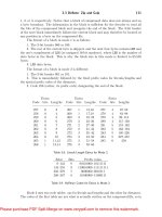
9 Solow model

113

Introduction 113
Economic model 113
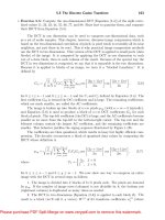
Numerical solution: initial value problems 119
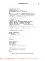
Computational implementation 121
Numerical results and simulation 122
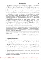
Highlights 125

Problems and computer exercises 127

10 Skill-biased technological change model

129

Introduction 129
Economic model 130
Numerical solution: initial value problems 134
Computational implementation 138
Numerical results and simulation 139
Highlights 141
Problems and computer exercises 142

11 Technological-knowledge diffusion model

143

Introduction 143
Economic model 144
Numerical solution: initial value problems 147
Computational implementation 150
Numerical results and simulation 151
Highlights 154
Problems and computer exercises 154

12 Ramsey–Cass–Koopmans model
Introduction 156
Economic model 156
Numerical solution: boundary value problems 163

Computational implementation 166
Numerical results and simulation 168
Highlights 170
Problems and computer exercises 170

156


x Contents

Afterword

173

PART III

Appendices
Appendix A: Projects

175
177

Supply–demand model with trade: export taxes 177
Product differentiation model 178
Some variants on the Mundell–Fleming model 180
Nonlinear supply–demand model 186
Dynamic continuous duopoly game 186
Dynamic IS–LM model 189
Dynamic AD–AS model 190
Extensions to the neoclassic growth model 191

Effects of public intervention on wage inequality 197
Migratory movements and directed technical change 199
Skill-structure, high-tech sector and economic growth dynamics model 200
Multiple equilibria in economic growth 204

Appendix B: Solutions

207

Supply and demand 207
IS–LM in a closed economy 209
IS–LM in an open economy 211
AD–AS 214
Portfolio 218
Supply and demand dynamics 222
Duopoly 228
SP–DG 229
Solow 234
Skill-biased technological change 239
Technological-knowledge diffusion 244
Ramsey–Cass–Koopmans 249
Bibliography
Index

257
261


Figures

I.1 Short–medium run stability
I.2 Long-run path: country with small growth rate (A) and with
high growth rate (B)
1.1 Supply and demand diagram
1.2 Consumer and producer surplus
1.3 Effects of a demand shock (negative)
1.4 Supply and demand curves for all markets
1.5 Supply and demand curves, with tariff, for all markets
1.6 Supply and demand curves, with subsidy, for all markets
2.1 IS–LM diagram
2.2 Decrease in T
2.3 Increase in G
2.4 Decrease in M
4.1 AD–AS diagram
4.2 Increase in G
4.3 Increase in M
4.4 Increase in A
5.1 Monte Carlo convergence path for the portfolio with
minimum variance
5.2 Efficient frontier, minimum variance portfolio, portfolio with
return equal to the asset with greater return and the assets
6.1 Cobweb plots
6.2 Price phase diagram for the inventory market model
7.1 Quantity phase diagram for the dynamic duopoly Cournot
game
8.1 SP-DG disinflation process
9.1 Solow diagram
9.2 Golden rule savings rate
9.3 Transition dynamics to steady state
9.4 Transition dynamics and Solow diagram: variation on δ

9.5 Transition dynamics and Solow diagram: variation on A
9.6 Direction field and paths to steady state
10.1 Path of variables D and W

xx
xxi
9
10
12
19
21
24
34
35
36
36
58
60
61
62
72
73
90
91
101
111
116
118
123
125

126
126
140


xii Figures

10.2
11.1
11.2
11.3
12.1
12.2
12.3
12.4
B.1

Path of variable D = Q H /Q L for several values of H
Transitional dynamics for Nˆ and χ2
Increase in ν2
Decrease in ν2
Golden rule, equilibrium point, steady state
Transition dynamics to steady state
Phase diagram, RCK model
Numerical estimates of the dynamic paths in the RCK model
Divergent processes (| − ab | ≥ 1)

141
151
152

153
162
169
169
171
224


Preface

There is consensus that computational approach to economics is a growing
field. The large majority of economists, or students in economics, are not
aware of numerical computing, although the ubiquity of numerical methods
is known. On the other hand, professionals or students in mathematics, physics
and engineering increasingly require economic knowledge.
This book blends economics with the numerical techniques required for
the solution of the problems, providing explained codes. It is precise and concise, meaning that it balances theory and practice. The textbook provides and
explains, with detail, the MATLAB/Octave implementation of the algorithms.
The intuition and central ideas of the numerical methods required to deal with
the mathematical theory underlying the economic problem are pedagogically
provided. The topics covered also prepare the reader to undertake more complex models and/or to develop new research. They give economic readers the
skills needed to understand the essentials about numerical methods to solve
economic problems, and provide more technical readers with an easy way to
cope with economics through modelling and simulation.
The main ingredients of the book are seminal economic models, relevant
and efficient numerical methods and (explained) software solutions. The aim
behind this choice is twofold. First, the book should be suitable for those who
do not have skills in either economics or in scientific programming. Second,
the book should be instructive, providing the basics and skills to deal with this
multidisciplinary topic.

Economic models A set of micro and macroeconomic models were selected

to be included in this book.
Regarding the short–medium run stability of the macroeconomic models, the
classical IS–LM model, in closed and open economy, is presented. Then the book
covers flexible prices and the determinants of inflation. Following on from the
former models, the AD curve from the IS–LM model is introduced along with
the short- and long-run AS curve. In addition, the SP–DG model to explain
the ups and downs of inflation is introduced. For the long-run macroeconomic
growth models, the book presents the seminal Solow model, which is extended
by the general equilibrium model called the Ramsey–Cass–Koopmans model.


xiv Preface

Two other models are also considered: one is a general equilibrium economic
growth model to explain the path of intra-country wage inequality; and the other,
a general equilibrium economic growth model as well, tackles the international
technological-knowledge diffusion from developed to developing countries.
The chapters on microeconomic models start by examining how the
behaviour of individual agents affect the supply and/or demand for goods
and services, which determines prices, and how prices, in turn, determine
the quantity supplied and/or quantity demanded of goods and services. The
proposed models meet exactly this outline, by first considering a static supply–
demand model, which is extended to consider international trade policy, and
then a dynamic cobweb model, which in turn is derived from the previous static
one. In this sequence, afterwards a dynamic duopoly game model, through
which firms compete by quantities, is analysed. Finally, to accommodate
optimisation problems, a portfolio model resulting from the setup originally
proposed by Markowitz is presented and solved using different approaches.

Numerical methods and software The economic models are presented
emphasising the underlying mathematical problems that must be solved. A
brief presentation of some of the most common and state-of-the-art numerical
methods to solve these problems is provided. Emphasis is given to numerical
methods to solve systems of linear and nonlinear equations, to solve systems of
differential equations (both initial and boundary value problems), and to solve
optimisation problems.
For the numerical implementation of the models as well as of the numerical
methods, MATLAB and Octave are used. Our choice was primarily based on
their adequacy for the purposes of the book, mainly due to ease of code writing,
availability of a plethora of functions programmed on state-of-the-art methods,
nice and rich plotting capabilities and ease of debugging.
MATLAB is a high-level language and interactive environment that enables
computationally intensive tasks. The codes were tested on several MATLAB
releases. A trial license can be obtained from the MathWorks (leading developer
of mathematical computing software for engineers and scientists) website. Additionally, MATLAB can be enlarged with toolboxes, which provide functions for
specific development areas.
GNU Octave is a high-level language, primarily intended for numerical
computations, mostly compatible with MATLAB. The codes were also tested
on the more recent Octave versions. It is freely redistributable software, under
the terms of the GNU General Public License (GPL) as published by the
Free Software Foundation. Octave-Forge provides a set of packages for GNU
Octave, to extend its functionalities.
To run the files provided in the book, the Optimization Toolbox is required for
MATLAB, and two packages, optim and odepkg, are needed for Octave. Some,
but few, functionalities may differ between the two software packages, but the
tendency is that newer versions of Octave tend to diminish these differences.

Preface xv
Project proposals The textbook proposes, at the end, a set of projects for
further development. These projects aim at consolidating and expanding the
skills gained as a result of studying this book.
Book prerequisites The textbook was conceptualised to be as much as possible self-contained. Some knowledge or at least general interest that the reader
certainly has of economics will prove helpful. It also helps to have some
mathematical background, mainly related to the basics of linear algebra and
calculus. Some familiarity with programming techniques may be advantageous.
A quick introduction to MATLAB (or Octave) programming is recommended
by reading one of the many short courses available in the world wide web.
Acknowledgments Many students assisted, by experiencing the contents of

this book and by preparing some reports, in the production of this book. We are
particularly grateful to Carlos Seixas, Diana Aguiar, Duarte Leite, José Gaspar,
Mariana Cunha, Pedro Gonzaga and Sofia Vaz for their efforts in preparing
outstanding reports that inspired some of the projects proposed in the book.
The influence of our colleagues at the Faculty of Economics was also
important: in particular, Pedro Gil for carefully reading some of the projects.
We acknowledge all anonymous referees for their careful reviews and valuable comments which helped to improve the manuscript. We would also like
to thank the Editor since without his professional procedure and helpful guidance this book never would have come to be produced in its present form. The
editorial team was also meticulous and unsurpassed.
The work of brilliant economists and mathematicians has been inspiring for
us, namely: Beresford Parlett, Cleve Moler, Daron Acemoglu, Gene Golub,
Mario Ahues, Robert Barro and Xavier Sala-i-Martin.
We would like to thank the Faculty of Economics at University of Porto
(FEP.UP) for believing and supporting our Computational Economics course
in the economics PhD program and our Numerical Methods course in the
MSc program.
We dedicate this book to our children, Nuno Vasconcelos, Ana Afonso,
Tiago Vasconcelos and João Afonso. We have always hoped to be an inspiration

to them, and still do. They are surely very inspiring to us.


Using the book

Notation Throughout this work, we generally adopt the Householder (1964)

notation. Greek letters indicate scalars, upper case letters indicate matrices and
lower case letters indicate vectors or scalar indices (namely, i , j , and k). For
vectors and matrices, subscripts are used in the following ways.
•
•
•
•

vk denotes a term in a sequence of vectors v0 , v1 , . . . , vk , vk+1 , . . ..
The element or component i of vector v is denoted by v(i ) (or simply by
vi when there is no conflict of notation with the previous convention).
Mk denotes a term in a sequence of matrices M0 , M1 , . . . , Mk , Mk+1 , . . ..
The element or coefficient in row i and column j of matrix A is denoted
by a(i, j ) (or simply by ai, j or ai j when there is no conflict of notation
with the first convention above).

A note to students We strongly advise students to replicate the codes provided

and to introduce slight modifications of the values of the parameters. Being
acquainted with the sensitivity of the numerical methods and economic models
is fundamental. We also encourage the development of some of the projects.
They follow an increasing level of difficulty, to cope with everyone’s needs
and pace.

A note to instructors The book can be used in several different types of
courses, such as the following.

•

Title: Introduction to Computational Macroeconomics (1 semester)
–

•

Syllabus: Chapters 2–4 and 8–12 plus some of the projects (Appendix A);
part of the course should be planned by the students to develop their
models or extend existing ones. Research skills regarding how to
investigate existing literature (books and papers) should be explored.

Title: Introduction to Computational Microeconomics (1 semester)
–

Syllabus: Chapters 1, 5–7 followed by some of the projects
(Appendix A); students are encouraged to plan and develop their


Using the book xvii

models taking into consideration the ones exposed. Research skills
regarding how to investigate existing literature (books and papers)
should be explored.
•

Title: Introduction to Computational Economics (1 semester)

–

•

Syllabus: Chapters 1–2, 4–7, 9 and some of the proposed projects
(Appendix A); part of the course should/could exploit further the
programming skills as well as the numerical methods.

Title: Topics on Computational Economics (1 semester)
–

Syllabus: Chapters 3, 8, 10–12 with emphasis in the projects
(Appendix A); the course should be complemented by dynamic programming models, either deterministic or stochastic, and optimisation
procedures.

We strongly recommend that the evaluation process should be performed
using modelling and computing assignments to be developed during the
semester. Two can be done individually and a third can be performed individually or in a small numbered group. Each assignment should be answered
in a report, following a working paper format, and presented briefly inside
the class room, so all students can profit from the work of their colleagues.
This methodology will enforce and strengthen the class cohesion as well as the
students’ capability and motivation to develop their own work, learning also
from others. The teacher should assume only an arbitrary role in this process,
allowing students to lead the presentations and the answers/responses period.
The teacher’s role, at least during these periods, should be to stimulate, mentor
and monitor; a course learner-driven instead of one teacher-driven should be
more appreciated by students allowing them to better stimulate their learning
pace.
Enjoy the book.

This page intentionally left blank


Introduction

The computational approach to economics is a growing field. Without this skill
it is not possible to simulate policy effects in today’s complex economic models.
However, there is a gap between the usual preparation in economics and the
computational tools. This book aims at bridging the gap between economics
and numerical computing. It enables economists or students in economics to
enrich their knowledge by endowing them with the required numerical and
computational skills. With equal interest, it allows the specialist in mathematics
and in computation to become familiar with economic problems.
The material covered gives the reader the skills needed to understand the
essentials about numerical methods to solve economic problems, by using standard economic models. The textbook provides and explains, with detail, the
MATLAB/Octave implementation of the algorithms. The intuition and central
ideas of the numerical methods required to deal with the mathematical theory underlying the economic problems are pedagogically provided. The topics
covered also prepare the reader to undertake more complex models and/or to
develop their own research.
The chapters are modular. They begin with a brief presentation of the economic problem, followed by its mathematical formulation and computational
implementation. As a result, the economic problem can be simulated in various
scenarios and therefore enables economic interpretation of the results. The reader
is challenged to modify the computational programs following proposals to change
the baseline models. Through this book, the reader acquires the necessary computational skills to understand and analyse economic models with ease, overcoming
limitations such as the size of the problem and/or the nonexistence of an explicit
solution. This skill may then be used to produce their own research.
The provided learning outcomes and competencies are thus: to offer a vision
of numerical methods in economics and its importance to the professional and
academic practice; to provide knowledge and understanding of concepts, methods, and application topics in numerical methods and computing relevant to

the economy; to support the development in the field of numerical methods
and economics, analytical skills, communication and learning appropriate to
the practice of the profession; to develop critical capacities, in particular in
modelling, analysis and treatment of data and results.


xx Introduction

real GDP

The book consists of two parts: the first deals with static economic models
and the second with dynamic economic models. Both parts incorporate macro
and microeconomic models, which are numerically solved. The required
numerical methods are presented throughout the book, illustrating how to solve
efficiently the models and providing the necessary knowledge to tackle other
problems with similar mathematical needs.
Macroeconomic themes dominate the news since directly or indirectly they
affect our well-being. Each of these themes involves the overall economic performance of the nation rather than whether one particular economic agent
earns more or less than another. Thus, macroeconomics deals with aggregate
economic variables.
In the short–medium run the three most important aspects are the output level,
the unemployment rate and inflation. More output level implies lower unemployment rate, but a higher rate of inflation (and vice versa). The output level
is measured by the real gross domestic product, GDP, which includes all currently
produced goods and services of an economy sold in the market in a certain time
period. The term real means that increases of the output reflect only increases
in the quantities produced; in general terms, a variable measured in real term
is free of changes in prices. It can be cast in actual (or effective) and natural (or
potential) real GDP. The former is the level indeed produced by an economy
and the latter is the real GDP when the inflation rate is constant. Figure I.1
illustrates the relations between these variables.

In this period of time, macroeconomists aim at minimising the fluctuations in unemployment and in the inflation rate, which requires also the
minimisation of real GDP fluctuations. Nevertheless, to achieve an increasing

natural real GDP
actual real GDP

natural unemployment rate
actual unemployment rate
time

inflation rate

unemployment rate

time

inflation rate
time

Figure I.1 Short–medium run stability.


Introduction xxi

natural real GDP
actual real GDP

real GDP

country B

country S

time

Figure I.2 Long-run path: country with small growth rate (A) and with high growth
rate (B).

standard of living the real GDP must grow, which is the long-run concern of
macroeconomists. Figure I.2 schematises two different economies with their
own gap between actual and natural real GDP but with different growth rates
(higher in economy B).
In turn, microeconomics analyses the market behaviour of individual consumers and firms in an attempt to understand the decision-making processes of
households and firms. It examines how these decisions and behaviours influence the supply and demand for goods and services, which determines prices,
and how prices determine the quantity supplied and demanded of goods and
services. Thus, it is concerned with the interaction between individual buyers
and sellers and the factors that affect the choices made by them. It includes
several areas: in particular, the supply–demand model of price determination
in a market, the consumer demand theory, the production theory, perfect
and imperfect competition, game theory, labour economics, international trade
policy, welfare economics and economics of information.
Specifically, the structure of the book is as follows. Part I, related to static
economic models, includes the following chapters.
•

Chapter 1 presents and solves a static supply–demand model, finding the
competitive economic equilibrium for price and quantity of a particular
good or service, which occurs when the quantity demanded by consumers
will equal the quantity supplied by producers. The model is extended to
include international trade policy and is solved by the Gaussian elimination

method, a direct method for linear systems.


xxii Introduction

•

•

•

•

Chapter 2 presents and solves the standard IS–LM model, which relates the
real output and the interest rate in the goods and services market (IS curve)
and in the money market (LM curve). Computations are then performed
through the LU factorisation (where L stands for lower and U for upper),
as part of the solution of systems of linear equations, introduced along with
stability issues.
Chapter 3 extends the previous IS–LM model to a scenario of an open
economy. As a result, the effects of both fiscal and monetary policies are
analysed in the setting of an open economy. An introduction to iterative
methods for the solution of linear systems is provided.
Chapter 4 introduces the AS–AD variable-price-level model. The AD
curve comes from the IS–LM equilibrium and the AS curve reflects the
labour market. Iterative numerical methods for the solution of nonlinear
systems of equations are introduced.
Chapter 5 is used to treat optimisation problems, by revisiting the problem
of portfolio optimisation originally proposed by Markowitz. The aim is to
implement a model that uses both a Monte Carlo optimisation and other

numeric techniques available in MATLAB/Octave.

Part II, dealing with dynamic economic models, comprises the following
chapters.
•

•

•

•

•

•

Chapter 6 deals with the dynamic cobweb model derived from the static
supply–demand model, by assuming that the supply reacts to price with
a lag of one period, while demand depends on current price. Numerical
computations for difference equations are presented.
Chapter 7 addresses the dynamic duopoly game model, through which
firms compete by quantities. The model allows us to analyse the strategic interaction between firms. The computational implementation provides additional insights into iterative processes and introduces numerical
methods for eigenvalue problems.
Chapter 8 explains the SP–DG model through which the dynamics of
inflation and output gap under disinflation strategies can be analysed, as
well as permanent demand shocks and temporary supply shocks. The
computational implementation provides insights to iterative processes.
Chapter 9 summarises the seminal Solow growth model, which highlights
a number of very useful insights about the dynamics of the growth process.
The Euler numerical method is presented to solve the related initial-value

problem.
Chapter 10 presents a dynamic growth model that explains the direction
of technological knowledge, which, in turn, drives intra-country wage
inequality. The Runge–Kutta family of numerical methods is used to reach
the solution of the respective initial value problem.
Chapter 11 analyses international technological-knowledge diffusion from
developed to developing countries through cheaper imitative R&D. As a


Introduction xxiii

•

result, developing countries grow more than developed ones during the
transitional dynamics phase towards the steady state. Numerical methods
with memory and methods to tackle stiff initial value problems are
mentioned.
Chapter 12 extends the Solow growth model in Chapter 9, by considering
an endogenous saving rate – the usually called Ramsey–Cass–Koopmans
model – which includes the rational behaviour of utility maximising
by individuals. To solve the boundary value problems for systems of
ordinary differential equations by the collocation method, some specific
MATLAB/Octave functions are referenced.

Finally, Appendix A proposes, through projects, either additional economic
models or extensions of the studied ones. These projects allow for knowledge
sedimentation, reflection on the topics covered, exploitation of new extensions
and features. Appendix B provides solutions for the proposed project exercises.

This page intentionally left blank