New models for sustainable logistics internalization of external costs in inventory management
Bạn đang xem bản rút gọn của tài liệu. Xem và tải ngay bản đầy đủ của tài liệu tại đây (6.62 MB, 111 trang )
SPRINGER BRIEFS IN OPERATIONS MANAGEMENT
Salvatore Digiesi
Giuseppe Mascolo
Giorgio Mossa
Giovanni Mummolo
New Models for
Sustainable Logistics
Internalization
of External Costs
in Inventory
Management
SpringerBriefs in Operations Management
Series Editor
Suresh P. Sethi
The University of Texas at Dallas, TX, USA
More information about this series at />
Salvatore Digiesi • Giuseppe Mascolo
Giorgio Mossa • Giovanni Mummolo
New Models for Sustainable
Logistics
Internalization of External Costs in Inventory
Management
Salvatore Digiesi
Department of Mechanics, Mathematics
& Management
Polytechnic University of Bari
Bari, Italy
Giuseppe Mascolo
Department of Mechanics, Mathematics
& Management
Polytechnic University of Bari
Bari, Italy
Giorgio Mossa
Department of Mechanics, Mathematics
& Management
Polytechnic University of Bari
Bari, Italy
Giovanni Mummolo
Department of Mechanics, Mathematics
& Management
Polytechnic University of Bari
Bari, Italy
SpringerBriefs in Operations Management
ISBN 978-3-319-19709-8
ISBN 978-3-319-19710-4 (eBook)
DOI 10.1007/978-3-319-19710-4
Library of Congress Control Number: 2015943587
Springer Cham Heidelberg New York Dordrecht London
© Springer International Publishing Switzerland 2016
This work is subject to copyright. All rights are reserved by the Publisher, whether the whole or part of
the material is concerned, specifically the rights of translation, reprinting, reuse of illustrations,
recitation, broadcasting, reproduction on microfilms or in any other physical way, and transmission or
information storage and retrieval, electronic adaptation, computer software, or by similar or dissimilar
methodology now known or hereafter developed.
The use of general descriptive names, registered names, trademarks, service marks, etc. in this
publication does not imply, even in the absence of a specific statement, that such names are exempt
from the relevant protective laws and regulations and therefore free for general use.
The publisher, the authors and the editors are safe to assume that the advice and information in this
book are believed to be true and accurate at the date of publication. Neither the publisher nor the
authors or the editors give a warranty, express or implied, with respect to the material contained herein
or for any errors or omissions that may have been made.
Printed on acid-free paper
Springer International Publishing AG Switzerland is part of Springer Science+Business Media
(www.springer.com)
Preface
Logistics of transport systems is a key driver for the growth of whatever economy.
Freight transport allows production systems or common citizens to receive or send
materials or finished goods required by processes as well as by everyday life
activities. Passenger transport, both public and private, allow people saving time
for their transfers and ensure high level of mobility. Materials and people journeys
fulfill economy and society expectations.
However, the overall transport sector accounts worldwide for more than half of
global liquid fossil fuels consumptions which, in turn, is responsible for a nearly
quarter of the world’s energy-related CO2 emissions, more than 80 % of air
pollution in the cities and about 1.3 million of fatal traffic accidents per year.
Negative effects represent ‘external costs’ paid by unaware societies and modern
economies.
Costs of externalities account worldwide for more than 10 % of the GDP with an
increasing trend. The European Environment Agency (EEA) and the United
Nations Environment Programme (UNEP) defined the ‘Avoid-Shift-Improve’
(ASI) strategy to tackle the increasing of externalities while EU Commission
(Directorate General for Mobility and Transport) established in 2011 a roadmap
that will lead to the internalization of external costs within 2020. Research
programs and strategic actions on sustainable development of smart cities are
focusing on smart mobility of goods and citizens due to the relevant
environmental, social and economic costs of logistics.
Internalization of cost of externalities gives rise to new logistics cost estimates and
functions which managers, researchers, lecturers and students should refer in
facing with logistics issues. Under this purpose the present book has been
conceived.
The book focuses on freight transports of industrial production systems. The most
used keywords are as follows: sustainable logistics, freight transport,
internalization of external costs, environmental cost, social cost, inventory
management, Economic Order Quantity—EOQ, logistics cost function, loss factor
of transport, Sustainable Order Quantity—SOQ, transport means selection,
stochastic variability of product demand, stochastic variability of supply lead time,
sensitivity analysis, finished vehicle logistics, inland waterways, automotive
supply chain, spare parts, repair policy.
The book has been subdivided into three main parts, organized as introduced
below.
v
vi
Preface
Chapter 1 provides a taxonomy of external cost figures as well as data set enabling
the reader to perform reliable estimates of freight transport external costs. To this
purpose, a full scale case study is developed.
Chapter 2 describes a new sustainable inventory management model whose cost
functions include externalities. The classical ‘Economic Order Quantity’ model is
re-formulated and the new concept of Sustainable Order Quantity (SOQ) is
defined.
Finally, in Chap. 3 the SOQ model is formulated for different inventory
management applications referred to both deterministic and stochastic production
environments. Numerical examples are provided.
We would like to thank our colleagues, both academics and professionals from
service companies, our students, and the editors at Springer for their valuable and
helpful support.
Bari (Italy)
Spring 2015
Salvatore Digiesi
Giuseppe Mascolo
Giorgio Mossa
Giovanni Mummolo
Contents
Preface ..................................................................................................................... v
List of Figures ....................................................................................................... ix
List of Tables ......................................................................................................... xi
About the Authors .............................................................................................. xiii
1
Internalization of External Costs of Freight Transport ........................... 1
1.1 Overview on the Transport System and the Legislative Context ............. 1
1.2 A Taxonomy of External Costs ................................................................ 4
1.3 A Case Study from Automotive Industry Logistics ................................. 9
1.3.1 Inland Waterway Transport (IWT) ................................................. 11
1.3.2 Discussion ....................................................................................... 15
References .............................................................................................................. 19
2
Sustainable Inventory Management ......................................................... 21
2.1 Notations ................................................................................................. 21
2.2 Overview of the State of the Art ............................................................. 23
2.3 The Loss Factor of Transport ................................................................. 26
2.4 A Sustainable Order Quantity (SOQ) Model ......................................... 29
2.4.1 Purchase and Ordering Costs .......................................................... 30
2.4.2 Transport Costs ............................................................................... 30
2.4.3 Holding Costs ................................................................................. 30
2.4.4 Shortage Costs ................................................................................ 36
2.4.5 External Costs ................................................................................. 37
References .............................................................................................................. 39
3
SOQ Model Formulations .......................................................................... 43
3.1 Deterministic Demand and Lead Time ................................................... 43
3.1.1 Environmental Costs ....................................................................... 45
3.1.2 Environmental and Social Costs ..................................................... 54
3.2 Stochastic SOQ Model ........................................................................... 66
3.2.1 Product Demand Uncertainty ......................................................... 67
3.2.2 Lead Time Uncertainty ................................................................... 76
3.2.3 SOQ of Repairable Spare Parts with Uncertain Demand ............... 84
References .............................................................................................................. 94
Index....................................................................................................................... 97
vii
List of Figures
Fig. 1.1 Gross Domestic Product, passenger and freight transport trend from
1995 to 2012 in EU28 ......................................................................................... 2
Fig. 1.2 External costs in EU27 in 2008 .................................................................. 5
Fig. 1.3 New passenger cars assembled worldwide from 2000 to 2013 ............... 10
Fig. 1.4 New passenger cars registered (or sold) worldwide from 2005
to 2013 ............................................................................................................... 10
Fig. 1.5: Overview of European inland Waterways .............................................. 12
Fig. 1.6: Heilbronn vessel ...................................................................................... 13
Fig. 1.7: Potential Countries for the distribution of the new passenger cars
in the Rhine-Main-Danube area ........................................................................ 13
Fig. 2.1 Different ways of transporting a load ........................................................ 27
Fig. 2.2 Loss factors of different transport means ................................................. 28
Fig. 2.3 Inventory level (I) over time in case of constant demand and
lead time ............................................................................................................. 31
Fig. 2.4 Inventory level (I) over time in case of stochastic demand ...................... 32
Fig. 2.5 Inventory level (I) in case of stochastic lead time (LT)
and LT = E(LT)................................................................................................... 33
Fig. 2.6 Inventory level (I) in case of stochastic lead time (LT)
and LT ≤ E(LT) ................................................................................................... 34
Fig. 2.7 Inventory level (I) in case of stochastic lead time (LT)
and E(LT) < LT ≤ LT* ........................................................................................ 34
Fig. 2.8 Inventory level (I) in case of stochastic lead time (LT)
and LT > LT* ...................................................................................................... 34
Fig. 3.1 Lot size (Q) vs. transport speed (v) ........................................................... 44
Fig. 3.2 Transport, environmental, holding costs and logistic cost
factor FL ............................................................................................................. 48
Fig. 3.3 FL values for different route lengths and f values ..................................... 49
Fig. 3.4 SOQ/G (a) and fOPT (b) versus transport distance L for different
p values .............................................................................................................. 50
Fig. 3.5 FL, SOQ/G, and fOPT values for ch = 5000 [€/tyear] in case of
(a) short distances (L = 400 [km]) and (b) long distances (L = 1000 [km]) ..... 51
Fig. 3.6 Specific logistics cost for different transport means and different
internalization strategies. ................................................................................... 63
Fig. 3.7 Specific logistics cost percentage increase compared to the
economic case for different transport distance (L) and two different
internalization strategies including all the external costs categories. ................ 64
Fig. 3.8 Specific logistics cost percentage increase compared to the economic
case for different transport distance (L) and two different internalization
startegies charging only GW and LCA external costs categories...................... 66
ix
x
List of Figures
Fig. 3.9 The supply chain of a multi-site manufacturing system. .......................... 69
Fig. 3.10 SOQ vs. cv values in case of L = 200 [km] and cS/ch = 0.65. .................. 75
Fig. 3.11 SS vs. cv values in case of L = 200 [km] and cS/ch = 0.65....................... 76
Fig. 3.12 Spare parts inventory level over time. ..................................................... 86
Fig. 3.13 Logistic cost factor (FL) vs loss factor (f) in case of = 0.5, = 0.9,
SL = 0.95, cv = 0.1, cR = cN, and p = 0.5 for different transport
distances (L) ....................................................................................................... 91
Fig. 3.14 Logistic cost factor (FL) vs. repair rate () in case of = 0.9,
SL = 0.95, cv = 0.1, and cR = cN for different transport distances (L)............... 92
Fig. 3.15 Logistic cost factor (FL) vs. repair rate () in case of = 0.9,
SL = 0.95, cv = 0.1, L = 500 [km] for different unit repair costs (cR) .............. 93
List of Tables
Table 1.1 Quantification of the potential passenger car flows in the
Rhine-Main-Danube area (year 2013) .............................................................. 14
Table 1.2 External costs of the freight transport [€cent/t·km] as in Marco
Polo Calculator .................................................................................................. 15
Table 1.3 CO2 and air pollutants (PM, SO2 and NOx) reduction for inland
vessels considering different fuel technologies ................................................ 16
Table 1.4 Number of new passenger cars transported (year 2013) ....................... 17
Table 1.5: External costs reduction of multimodal transport ................................ 18
Table 2.1 Notations adopted .................................................................................. 21
Table 2.2 Loss factor (f) value for different means of transport (data 2009) ........ 28
Table 2.3 Loss factor (f) value for different means of transport (data 2012) ........ 29
Table 2.4 Expected inventory level and ordering cycle length in the three
cases considered ................................................................................................ 36
Table 3.1 Es, f, ei, and vACT values for different means of transport ...................... 46
Table 3.2 Results of the regression analysis .......................................................... 47
Table 3.3 Parameters values of Eq. (3.10) ............................................................. 48
Table 3.4 Allowable lead time (LTALL) values obtained by the model
in case of p = 0.5 (k = 0.5; ch = 5000 [€/tyear]) .............................................. 52
Table 3.5 Solutions of the logistics problem (36) in case of L = 400 [km]
(k = 0.5; ch = 5000)........................................................................................... 53
Table 3.6 Solutions of the logistics problem (36) in case of L = 300 [km]
(k = 0.5; ch = 5000 [€/tyear]) ........................................................................... 53
Table 3.7 Unit external costs [€2013/t·km] of different transport means ................ 54
Table 3.8 Loss factor (f) and average speed of transport (v) values for
different means of transport; [DB1] = [1], 2012; [DB2] = [6], 2012;
[DB3] = [7], 2007; [DB4] = [8], 2012. ............................................................ 55
Table 3.9 UK statistics adopted (year 2011) ......................................................... 57
Table 3.10 Average values of the loss factor for different transport
modalities .......................................................................................................... 58
Table 3.11: Data set adopted for the numerical experiment .................................. 59
Table 3.12 FL,ECON and FL,SUST for different transport distances ............................ 60
Table 3.13 SOQECON and SOQSUST for different transport distances...................... 60
Table 3.14 rECON and rSUST for different transport distances .................................. 60
Table 3.15 : Sustainable Order Quantity (SOQ) for different transport
means and distances .......................................................................................... 61
Table 3.16 : Reorder level (r) for different transport means and distances ........... 61
Table 3.17 Percentage increase of the specific logistics cost for different
internalization strategies compared to the economic case (External costs
charging level = 0 %) ....................................................................................... 62
xi
xii
List of Tables
Table 3.18 Percentage increase of the specific logistics cost in case of
different internalization strategies charging only GW and LCA external
costs categories compared to the economic case (External costs charging
level = 0 %)....................................................................................................... 65
Table 3.19 ei values for different means of transport ............................................ 70
Table 3.20 Classification factors adopted .............................................................. 70
Table 3.21 Regression parameters and unit monetary costs for the impact
category considered........................................................................................... 71
Table 3.22 Transport cost data adopted ................................................................. 72
Table 3.23 Regression parameters values of transport costs functions ................. 72
Table 3.24 Results obtained in case of cS/ch = 0.65 .............................................. 73
Table 3.25 Results of the cS/ch sensitivity analysis in case of L = 200 [km] ........ 75
Table 3.26 Expected inventory level and ordering cycle length in the three
cases considered ................................................................................................ 77
Table 3.27 Parameters values for unitary transport cost evaluation per
transport distance .............................................................................................. 80
Table 3.28 Sustainable and economic solutions comparison in case of cv = 0..... 80
Table 3.29 Optimal means of transport (fOPT) and SOQ values for different
L and cv values in case of SL = 0.95................................................................. 81
Table 3.30 Reorder level (r(fOPT)), SS, and FL values for different L and cv
values in case of SL = 0.95 ............................................................................... 82
Table 3.31 Optimal loss factor (fOPT) values of the sustainable and of the
economic (EX = 0) solution............................................................................. 82
Table 3.32 SOQ values for different L, cv, and cO values in case of SL = 0.95 .... 83
Table 3.33 Further notations adopted in the SOQ model of reparable spare
parts ................................................................................................................... 84
Table 3.34 Parameters values adopted................................................................... 89
Table 3.35 EOQ and SOQ model results comparison ........................................... 89
Table 3.36 SOQ model results in case of L = 200 [km] and cR = cN .................... 91
Table 3.37 SOQ model results in case of L = 500 [km] and cR = cN .................... 91
Table 3.38 SOQ model results in case of L = 1000 [km] and cR = cN .................. 92
About the Authors
Salvatore Digiesi. Graduated in Mechanical Engineering at the Polytechnic of
Bari—Italy. European Ph.D. in “Advanced Production Systems” at the
Interpolitecnica School of Doctorate. Tenured assistant professor of mechanical
plants at the Polytechnic of Bari. Member of the Board of Professor of the Ph.D.
Course on “Mechanical and Management Engineering” at the Polytechnic of Bari.
His main research topics are sustainable production and logistics, human
performance modelling, and energy recovery systems from biomasses.
Giuseppe Mascolo received his master’s degree in Mechanical Engineering in
2011 at the Polytechnic of Bari and the second level master’s degree in “Industrial
Plant Engineering and Technologies” in 2012 at the University of Genoa, both
with full marks. He is pursuing his Ph.D. in “Mechanical and Management
Engineering,” with a focus on Sustainable Logistics, at the Department of
Mathematics, Mechanics and Management (DMMM) of the Polytechnic of Bari.
Giorgio Mossa. He earned a degree in Mechanical Engineering and a Ph.D. in
“Advanced Production Systems Engineering” at the Polytechnic of Bari. He got a
master in “Energy and Environmental Management and Economics” at the School
“E. Mattei”—ENI Corporate University. In 2014 he earned the National Scientific
Qualification for the University Associate Professor position. Tenured assistant
professor of operations management and industrial systems engineering and
member of the Board of the Ph.D. Course on “Mechanical and Management
Engineering” at the Polytechnic of Bari. Main research topics are environmental
management of production systems, human performance modelling, design and
management of industrial systems, risk, safety and security management.
Giovanni Mummolo is full professor of graduate and postgraduate industrial
engineering courses at the Polytechnic of Bari (Italy), Department of Mechanics,
Mathematics, and Management. His main fields of research are in production
management and system design. He is responsible for several international research
projects and is referee of many international journals. He received the Research
Award of the CIO 2014-ICIEOM-IIE International Conference. He is President of
the European Academy for Industrial Management.
xiii
1 Internalization of External Costs of Freight
Transport
Abstract
Accidents, global warming, congestion, air pollution and noise are examples of
negative effects related to the transport activities that generate costs not fully
borne by the transport users and hence not taken into account when they make a
transport decision: these are the so called external costs. The internalization of the
external costs of transport has been an important issue for transport research and
policy development for many years worldwide. This Chapter, starting from an
overview of the transport sector statistics and of transport external costs
internalization in Europe, gives a taxonomy of the main transport external costs;
moreover, the state of art on the cost estimation methodologies is briefly
introduced. A case study from the finished vehicle logistics in the automotive
sector is presented. Results show the potential external costs reduction due to the
better environmental and social performance assured by the modal shift from
road toward inland waterways transport.
Keywords: Sustainable logistics, Freight transport, Internalization of external
costs, Environmental cost, Social cost, Finished vehicle logistics, Inland
waterways
1.1
Overview on the Transport System and the Legislative
Context
The transport sector, including the movement of people and goods by cars, trucks,
trains, ships, airplanes, and other vehicles, is a key drive for the European Union
Countries economic growth. It accounts for about the 5 % of the EU28 Gross
Value Added (GVA) and employs about the 5 % of the total workforce in the
EU28 [1]. In 2012, freight transport activities amounted to 3768 billion [t·km]
while passenger transport ones to 6391 billion [p·km]. Figure 1.1 shows the 1995–
2012 data of the Gross Domestic Product (GDP), of the freight transport and of the
passenger transport in EU28 [1] (year 1995 values: 8012 billion [€] for the GDP,
3.07 billion [t·km] for the freight transport and 5.37 billion [p·km] for the
passenger transport).
© Springer International Publishing Switzerland 2016
S. Digiesi et al., New Models for Sustainable Logistics,
SpringerBriefs in Operations Management, DOI 10.1007/978-3-319-19710-4_1
1
2
1
In
nternnalizzatioon off Ex
xternnal Costs
C s off Freightt Traanspport
Fig. 1..1 Gross
G s Dom
mesttic Produ
P uct, passsengger and freigh
f
ht trranspport trennd fro
om 119955 to 2012
2 2 in
E
EU228 [11]
U ortu
Unfo
unateely trannspoort sect
s tor, chaaracterizedd maainlyy byy foossill fueel drriveen m
moto
or
vehi
v icless, givess risse too neegattive effe
fectss.
This
T s secctorr, w
world
dwidde, is reespoonsiblee of::
m
moree thaan half
h of gglob
bal lliquuid foss
f sil fu
uelss connsuumpttionn;
neearlly a quaarterr off thee woorldd’s ener
e rgy--relaatedd CO
O2;
m
moree thaan 80
8 % of th
he aiir poolluutionn in citiies in
i deve
d elopping cou
untrries;;
m
moree thaan 1.27
1 7 million faatal trafffic acccidennts per yeaar;
chhron
nic ttrafffic conngesstionn in maany of the
t w
worrld’ss urb
bann areeas.
These negativve effects cause costs, whiich can add up to morre thhann 10 % of a
coun
c ntryy’s Gro
G oss Dom
D messtic Prooducct, ppaidd byy thhe soci
s iety andd arre llikely to
t ggrow
w,
prim
p marily beccausse oof the
t
expeccted grrowtth of the globaal vehi
v icle fleeet. Th
he
cont
c tinuuatio
on oon a buusinness-as--usu
ual ppathh will
w resu
r ult iin an
a increeasee off th
he globaal
vehi
v icle fleeet fr
from
m aroounnd 800 m
milllionn to betw
weeen 2 annd 3 billlion
n byy 2050. Moost of
o
groowth
this
t
h w
will be conncen
ntratted in the devveloopin
ng ccounntriees. Furrthermo
ore, it is
also
a
exppected an expponeentiiallyy grrowtth for
f the
t aviiatioon secto
s or (mai
( inlyy du
ue too th
he
deve
d elopping
g coountriess) annd a grrowtth bby up
u too 2550 % of thhe caarbo
on eemissio
ons from
m
ship
s ppinng [2
2].
T shiift ttowaard a gree
The
g en ttran
nspoort is
i need
n ded. EE
EA andd UN
NEP
P pprop
poseed an
a
holi
h stic strrateggy, callled the Avvoid
d-Shhift--Impprovve (AS
( I) strat
s tegy
y [2], too reeachh this
goal
g l. Thhe ASI
A straateggy aims
a s at::
1.
2.
3.
ding or redu
r ucinng th
he nnum
mberr off jou
urneeys take
t en;
avvoid
shhiftin
ng tto more
m e enviro
onm
menttallyy eff
fficieent form
ms of
o trranssporrt;
im
mpro
ovinng vehic
v cle and
d fueel teechnnoloogy..
1.1 Overview on the Transport System and the Legislative Context
3
In this context it can be included the external costs internalization strategy.
The European Commission focused the attention on the external costs of the
transport for many years and, in 1995, defined the transport externalities as
follows [3]:
“Transport externalities refer to a situation in which a transport user either does
not pay for the full costs (e.g. including the environmental, congestion or accident
costs) of his/her transport activity or does not receive the full benefits from it.”
The aim of the external costs internalization is the integration of these costs in
the decision making process of the transport users [4]:
directly: through, for example, command and control measures;
indirectly: through market-based instruments providing the right
incentives to the transport users such as, for example, taxes, charges and
emission trading;
by combinations of these basic types: for example, existing taxes and
charges may be differentiated by the EURO emission classes of vehicles.
The use of market-based instruments is generally regarded as the best strategy
to limit the negative effects of the transport requiring, however, a detailed and
reliable estimation of external costs. In order to better define the external costs it is
important to highlight the difference between:
social costs: reflect all costs occurring due to the provision and use of
transport infrastructure (i.e. wear and tear costs of infrastructure, capital
costs, congestion costs, accident costs, environmental costs);
private (or internal costs): directly paid by the transport users (i.e. wear
and tear and energy cost of vehicle use, own time loss costs, transport
fares, and transport taxes and charges).
As aforementioned, the European Commission has pointed out the objective to
charge the vehicles for the external costs they generate since 1995 [3]. European
Directive 1999/62/EC [5] (also called Eurovignette-Directive) and its amendment
[6] are consistent with this goal. European Directive 1999/62/EC did not includ
all the transport means but was limited to vehicle taxes, tolls and user charges
imposed on heavy duty vehicles (HDVs) aiming at the harmonization of levy
systems and at the establishment of a fair mechanism for charging the
infrastructure costs on vehicles using them. The spatial scope of this directive was
the Trans-European Transport Networks (TEN-T), a planned set of road, rail, air
and water transport networks to improve the transport sector performance in the
European Union. The Directive already recognized, in a general way, the
possibility to address a certain amount of the toll revenues to environmental
protection activities but the main destination of the tolls revenues was only the
recovering of the infrastructure costs (costs of construction, operation and
maintenance). By adopting only the user pays principle, this Directive failed in
recognizing also the polluter pays principle: all road users were considered alike
without considering for example the different congestion or pollution they caused.
4
1 Internalization of External Costs of Freight Transport
Furthermore, the spatial limitation to the TEN-T may cause a traffic shift towards
not charged networks. In 2011, the Council adopted the new EurovignetteDirective [6] acting on all Member States’ motorways and not only on the TEN-T.
Each Member State may define tolls composed of an infrastructure charge that
considers also the negative effect of traffic congestion, and/or an external-cost
charge related to traffic-based externalities (e.g.: air and noise pollutions). Only
suggestions and not obligations are provided regarding the use of the revenue from
infrastructure and external costs.
The internalization of the external cost is treated also in the EU White Paper in
2011 [7]: this document comprises 40 initiatives to be actuated within 2020 in the
EU. The ‘smart pricing and taxation’ initiative is divided into two phases. The first
phase, up to 2016, expects to start with a mandatory infrastructure charging for
HDVs and to proceed with the internalization of the external costs for all modes of
transport. The second phase, from 2016 until 2020, expects to implement a full
and mandatory external costs internalization for road and rail transport and to
examine a mandatory internalization of the external costs on all European inland
waterways network. The mandatory external costs internalization could also help
achieving other objectives included in the White Paper such as shifting: (i) 30 %
of road freight over 300 [km] to other modes such as rail or waterborne transport
by 2030 and more than 50 % by 2050; (ii) the majority of medium-distance
passenger transport from road to rail by 2050.
1.2
A Taxonomy of External Costs
According to the most recent estimates, the total external costs of transport in the
EU27 countries (with the exception of Malta and Cyprus but including Norway
and Switzerland) in 2008 have been estimated at about 500 billion [€], excluding
congestion, and at about 700 billion [€] including congestion. The GDP in EU27
in 2008 was about 12.5 quadrillion [€]: the total impact of externalities amounted
to 5–6 % of GDP. Fig. 1.2a shows that accidents, congestion, climate change and
air pollution represent 86 % of total costs. Moreover (see Fig. 1.2b), the road
sector generate 93 % of total external costs, rail accounts for 2 %, the aviation
passenger sector 4 % (only continental flights), and inland waterways 0.3 % [8].
In the following, for each cost category, the type of cost figures considered and the
methodologies for their estimation are pointed out.
1.2
A Taxxonoomy of Exte
E ernall Co
osts
5
Fig. 1.22 Extternaal coosts in
i EU27
7 in 220088 [8]]
Acc
A cideentt Coostss
T exteernaal accciddentt costs are relaatedd to the cossts nnot covvered byy thhe in
The
nsurrancce
prem
p mium
m suchh as,, forr exxam
mple, paain aand suffferiing cauusedd byy thee traafficc accciddentts.
The
T besst ap
pprooach too esstim
mate thee maargiinal acccideent eexteernaal co
osts is the
t botttom
masssum
up
u meth
m hod
dologgy. Thee main
m
mptioon of
o thhis app
a roacch is
i thhat whe
w en thhe driv
d ver of
o
an
a add
a ition
nal vehiclle join
j ns thhe trafffic expposes him
mself/heerself tto the
t aveerag
ge
acci
a dennt riisk. Thiis aaverragee accideent riskk caan be
b estim
e mateed thro
t oughh thhe sttatissticaal
relat
r tionnship
p beetweenn thee nu
umbber of
o aaccidennts invo
olvinng a giiven
n veehiclle class
c s an
nd
the
t traf
t ffic flow
w obse
o erved in
n thhe prev
p iouss yeearss. Th
he ccostts reelatted tto the
t acciden
nt
risk
r aree:
•
he eexpeecteed coostss, foor th
he persoon expo
e osed
d to thee risk, of
o deeathh an
nd innjurry
th
due
d tto an
a accciddentt;
th
he eexpeecteed costss foor th
he reelativess annd frien
fr nds of the personn exp
posed to
th
he rrisk;;
6
1
Internalization of External Costs of Freight Transport
•
accident cost for the rest of the society (material costs, police and
medical costs, output costs).
The concept of the Willingness To Pay (WTP) for safety is used to evaluate the
first two cost elements focusing on the Value of a Statistical Life (VSL) [4]. The
estimates on the VSL generally come from studies where participants to these
studies quantify own WTP for the reduction of the accident risk. These estimates
are different across countries, age groups and also differ from the risk analyzed: in
fact, the expected number of life years lost differs among different risk cases.
Several approaches could be adopted to quantify the share of the external costs
in total accident costs taking into account what is already covered by the insurance
of the person exposed to risk [4].
Climate Change Costs
Climate Change (or Global Warming) impacts of transport are mainly related to
the emissions of the greenhouse gases such as carbon dioxide (CO2), methane
(CH4) and nitrous oxide (N2O). In the case of aviation, at high altitude, also other
emissions (water vapor, sulfate, soot aerosols and nitrous oxides) have an impact
on global warming. Several methodologies are available to estimate the climate
change costs for the different transport modality: the state-of-art approach for
evaluating this externality is the damage costs approach called Impact Pathway
Approach (IPA) characterized by the following main steps:
•
•
•
quantification of the GHG emission factors, in [(CO2)eq] for different
vehicles;
valuation of climate change costs per tonne of [(CO2)eq];
calculation of the marginal climate change costs for different vehicle and
fuel types.
The damage cost approach and the abatement cost approach are the two main
methodologies evaluating the cost of the GHG emissions [4]. The first one
evaluates the total costs supposing that no efforts are taken to reduce the GHG
emissions; the second one evaluates the costs of achieving a certain amount of
emissions reduction. Between the two methodologies the abatement cost approach
is preferred, although the damage cost approach is desirable from a scientific point
of view; at the same time it is characterized by a high uncertainty mainly because
it is not possible to identify and to evaluate many risks related to future climate
change costs. The abatement costs approach mainly reflects the willingness-to
pay, of a society, for a certain abatement level of the emissions. In the abatement
costs evaluation, usually two different targets are considered in Europe:
1.
EU Greenhouse gases emissions reduction target for 2020 (corresponding
to a cut of 20 % of GHG emissions compared to 1990 levels, “low
scenario”);
1.2
2.
A Taxonomy of External Costs
7
a longer term target for keeping concentration of CO2eq in the atmosphere
below 450 [ppm] (thus keeping global temperature rise below 2 [°C]
relative to pre-industrial levels [9], “high scenario”).
Congestion Costs
The concept of congestion externalities is easily understandable but difficult to
quantify. A road network user affects, by his/her decision to use a certain network
for driving between two different destinations, the utility of all other users who
want to use the same network. The utility loss, aggregated over all those other
users, is the negative external effect of the respective user’s decision to move
between the same destinations. The utility loss is translated into costs considering
the willingness to pay for avoiding this utility loss. Thus, the external effect is
measured in terms of a monetary amount per trip.
The update of the unit values for congestion costs, suggested by the last
“Handbook on the external costs” commissioned by the European Commission
[4], is based on the aggregated approach of the FORGE model used in the
National Transport Model of the United Kingdom [10].
Air Pollution Costs
Air pollution costs are mainly due to the emission of air pollutants such as
particulate matter (PM10, PM2.5), nitrogen oxides (NOx), sulfur dioxide (SO2),
ozone (O3) and Volatile Organic Compounds (VOC). The following effects are
related to this externality:
•
•
•
•
health costs. Impacts on human health due to the aspiration of fine
particles (PM2.5/PM10, other air pollutants). In addition, also Ozone
(O3) has impacts on human health;
building and material damages. Mainly two effects have the most
impact: (1) soiling of building surfaces/facades mainly through
particles and dust; (2) degradation on facades and materials through
corrosive processes due to acid air pollutants like NOx and SO2;
crop losses in agriculture and impacts on the biosphere. Acid
deposition, ozone exposition and SO2 damage crops as well as forests
and other ecosystems;
costs for further damages for the ecosystem. Eutrophication and
acidification due to the deposition of nitrogen oxides as well as
contamination with heavy metals (from tire wear and tear) impact on
soil and groundwater.
The unit cost estimation of the air pollution for the different transport
modalities follows the already mentioned Impact Pathway Approach aiming, in
this case, at the quantification of the impact of the emissions on human health (the
major effects), environment, economic activity, etc. [4]. The key steps of the IPA
are the:
8
1
Internalization of External Costs of Freight Transport
determination of the burden of pollutants (e.g. by using vehicle emission
factors);
modeling of the dispersion of the pollutants around the source;
exposure assessment to evaluate the risk of the population exposed to the
defined burdens;
evaluation of the impacts caused by the pollutants to the human health
and to the environment;
monetary quantification of each impact (this step is usually based on the
willingness to pay for reduced health risks).
Costs of Up and Downstream Processes
This costs category considers the external costs generated by indirect effects
(not related to the transport journey itself) such as the production of energy,
vehicles and transport infrastructure. These costs occur also in other markets, such
as the energy market, in addition to the transport one so it is important to consider
the appropriate level of internalization within these markets. The most relevant
cost categories considered in [4] are:
energy production (well-to-tank emissions—WTT);
vehicle production, maintenance and disposal;
infrastructure construction, maintenance and disposal.
The methodology adopted to calculate these costs is basically founded on the
air pollution and climate change external costs estimation. The various studies
treating this argument differ, among them, from the cost categories covered: for
example some studies consider only the climate change costs of the up- and
downstream processes whereas others also considers costs related to the air
pollution costs.
Noise Costs
Exposure to noise emissions from traffic causes not only disturbs to people but it
can affect their quality of life and health. The greater urbanization and the increase
in traffic volumes are increasing the noise emissions. The two major negative
impacts associated to this externality are:
costs of annoyance: due to social disturbances of persons exposed to
traffic noise which result in social and economic costs such as discomfort
and pain suffering;
health costs: noise level above 85 [dB(A)] can cause hearing damage
while lower level (above 60 [dB(A)] may result in changing of heart beat
frequency, increasing of blood pressure and hormonal changes.
Furthermore, noise exposure can increase the risk of cardiovascular
diseases and decrease the quality of sleep.
1.3
A Case Study from Automotive Industry Logistics
9
The most used methodology to estimate the marginal noise external costs is
the Impact Pathway Approach. The key steps of the IPA [11] are:
level of noise emissions measured in terms of change in time, location,
frequency, level and source of noise;
noise dispersion models used to estimate the changes in the exposure to
noise according geographical locations, and measured in dB(A) and noise
level indication;
Exposure-Response Functions (ERFs) showing a relationship between
decibel levels and negative impacts of the noise;
economic valuation techniques of the negative impacts of the noise
identified;
overall assessment to identify aggregated economic values taking into
account all the negative impacts identified.
Other External Costs
The researches on the external costs, generally, focus only on the most
important cost categories costs (such as air pollution costs, noise costs, climate
costs or accident) neglecting other external costs categories. The reasons are
mainly due to the complexity in the impact pattern and uncertainty in the valuation
approaches. Methodologies for the calculation of these external costs are present
only in few studies thus, presently, are not as sophisticated as for the most studied
external costs categories [4]. The other external costs categories estimation
considered are: costs for nature and landscape, cost to ensure water and soil
quality, costs to ensure biodiversity losses, cost in urban areas (such as separation
costs for pedestrian and costs of scarcity for non-motorized traffic).
1.3
A Case Study from Automotive Industry Logistics
Worldwide, 65,462,496 passenger cars have been assembled and 62,786,169
registered (or sold) in 2013. Fig. 1.3 shows the worldwide passenger cars
production from 2000 to 2013 [12] by macro-areas while Fig. 1.4 shows the
worldwide passenger cars registrations (or sales) from 2005 to 2013 [13].
10
1 Interrnaliizatiion of Exterrnal Cossts of Frreighht Trranssportt
F 1.3 New
Fig.
w passennger carss assemb
bled worrldwiide from
f m 20000 too 2013 [ownn Figgure baseed on
n
[[12] dataa]
w paassenngerr carss reggisteered (or sold)
s ) woorldw
wide from
m 20005 to
t 20013 [ow
wn Fiiguree
Fig.. 1.4 New
based
b d on [13]] datta]
A widesspreead anaalysis cove
c ering
g thhe Euro
E ope hass been con
c nduccted to iden
ntify
fy th
he
flow
f ws oof the
w ppassseng
ger carrs ffrom
m thhe asseembbly plaants to each nationaal
t new
Euro
E opeaan mar
m rket.. Thhe main
m n steeps followeed to
t peerfo
orm thee anaalyssis hhavee beeen:
Paasseengeer caars defi
finitiion.. Acccorrdinng to
o Euurosstat [14
4] aand OIC
CA [15],
a ppassengger carr is a moto
m or vehi
v cle witth aat leeast fou
ur w
wheeels use
u d fo
or
mum
m ninne pass
p seng
gers inccludding thee driiverr.
thee traanspportt of maaxim
1.3
1.3.1
A Case Study from Automotive Industry Logistics
11
o aautom
mottivee assem
mbly
y pllants inn Europe. Mo
ore thaan
Identiificaation of
p engger cars
c s asssem
mbly plaants hav
ve bbeenn identiifiedd inn thee Euurop
pe
1000 pass
exxcludingg Ruussiia [16]..
Identiificaation off neew pass
p sengger car mo
odelss asssem
mbleed inn eaach plannt. A
weeb-rreseearchh perfo
p orm
med on thee Orig
O inall Eqquippmeent Maanuffactturerrs
offficial w
webssites alllow
wed idenntify
fyingg th
he caar mod
m dels asseembbled
d in eacch
plaant.
Collection of new passenger cars registration statistics in 2013 for the
European Countries. These statistics have been found in public
databases and, for some Countries, contacting privately national
statistics associations. The statistics are split by passenger cars model.
Quantification of the new passenger cars flows from the assembly
plants to the selected countries. The passenger cars distribution flows
have been calculated by crossing the data collected in the previous
steps. Each model assembled only in one plant (for example the Dacia
Logan assembled only in the Romanian plant of Colibasi) provided
quite certain information about the related distribution flows origin. In
some cases, in 2013, a car model has been assembled in more than one
plant (for example Audi A4 assembled in the German plants of
Ingolstadt and Neckarsulm): it has been made the assumption that in
each European country the 50 % of the Audi A4 flow came from
Ingolstadt and 50 % from Neckarsulm. More accurate hypotheses
have been made if available the total number of the cars assembled in
the plants split by model. For example Opel Astra, in 2013, has been
assembled in Gliwice (Poland), Rüsselsheim (Germany) and Bochum
(Germany) plants, respectively 100,886, 58,547 and 16,339 units. The
flows in this case have been split in proportion to the number of cars
assembled in these three plants.
Inland Waterway Transport (IWT)
The European Union is characterized by a network of inland waterways of more
than 40,000 [km] [1], 29,172 [km] of which have been earmarked by
Governments as waterways of international importance [17]. The most important
European waterways are located in the South-East corridor, East-West corridor,
Rhine corridor and North-South corridor (Fig. 1.5). As aforementioned, inland
waterway transport accounted in the EU28, in 2012, only for 4 % of freight
transport based on tonne-kilometres [t⋅km] [1].