Forecasting of black pepper price in Karnataka state: An application of Arima and arch models
Bạn đang xem bản rút gọn của tài liệu. Xem và tải ngay bản đầy đủ của tài liệu tại đây (591.54 KB, 11 trang )
Int.J.Curr.Microbiol.App.Sci (2019) 8(1): 1486-1496
International Journal of Current Microbiology and Applied Sciences
ISSN: 2319-7706 Volume 8 Number 01 (2019)
Journal homepage:
Original Research Article
/>
Forecasting of Black Pepper Price in Karnataka State: An Application of
ARIMA and ARCH Models
H.B. Mallikarjuna1*, Anupriya Paul1, Ajit Paul1, Ashish S. Noel2 and M. Sudheendra3
1
Department of Mathematics and Statistics, 2Department of Agricultural Economics,
SHUATS, Allahabad, India
3
Department of Agriculture Extension, College of Agriculture, UAHS, Shivamogga, India
*Corresponding author
ABSTRACT
Keywords
Forecasting, Price,
Black Pepper,
ARIMA, ARCH,
GARCH
Article Info
Accepted:
12 December 2018
Available Online:
10 January 2019
The study was conducted to forecast the price of black pepper in one of the major markets
of Karnataka state as the state ranks first position in production of pepper in India. The
Gonikoppal market in Kodagu district was selected purposively on the basis of highest
area and production in the state. The monthly prices of black pepper in Gonikoppal market
were collected from the Karnataka State Agricultural Marketing Board, Bangalore,
Karnataka state for the year 2008-09 to 2017-18. The time-series models such as ARIMA
and ARCH models were applied to price data using software’s such as SPSS, Gretl and
EViews. The Augmented Dickey-Fuller test and Heteroscedasticity Lagrange’s Multiplier
test were used to test the stationarity and volatility of the time-series respectively. The best
forecasted model was determined based on the lowest values of Akaike’s Information
Criterion (AIC) and Schwartz Bayesian Information Criterion (SBIC). However, the
predictability power, performance and quality of the model was measured based on the
lowest error value of the Root Mean Square Error (RMSE) and Mean Absolute Prediction
Error (MAPE). Among the tested models the prediction accuracy of the ARIMA model
was higher than ARCH family models. On the basis of the results, the ARIMA (0,1,1)
provide a good fit for forecasting the price of black pepper.
Introduction
Black pepper is an important spice crop in the
Karnataka state. The analysis of price over
time is important for formulating a sound
agricultural price policy. Agricultural prices
give the signal to both producers and
consumers regarding the level of production
and consumption. Changes in the relative
prices of the various agricultural commodities
affect the allocation of resources among
agricultural commodities by the producers.
Agricultural price movements have been a
matter of serious concern for policy makers in
our country as the behaviour of agricultural
prices adversely affects the steady economic
development. Among other things, price plays
a strategic role in influencing the cultivation
of pepper. Indeed, the price analysis of pepper
assumes greater significance not only to the
1486
Int.J.Curr.Microbiol.App.Sci (2019) 8(1): 1486-1496
policy makers but also to producers and
consumers. The black pepper prices have been
highly fluctuating over the years. An increase
in price of pepper affects the consumer by way
of increase in food consumption budget, while
a decrease in pepper prices below the cost of
cultivation affects the producer. No studies
have been conducted on forecasting the price
of black pepper so far. In this context, it is
necessary to know to what extent the prices
are being fluctuated and to draw meaningful
policy conclusion. Hence, the study focuses on
the objective to forecast the black pepper price
by using various time-series models.
Bhardwaj et al., (2014) applied the ARIMA
models and GARCH models for forecasting
the spot prices of Gram at Delhi market. They
were procured the secondary data for a period
of 01 January 2007 to 19 April 2012 from
NCDEX website. The AIC and SIC values
from GARCH model were smaller than that
from ARIMA model. Therefore, the GARCH
(1,1) model was found better model in
forecasting spot price of Gram.
Seyed Jafar Sangsefidi et al., (2015) applied
the ARIMA models and GARCH models for
forecasting the prices of agricultural products,
including potato, onion, tomato and veal. The
results of the ARIMA model and ARCH
models were compared. The results showed
that the estimation due to ARIMA method has
less relative error than the estimation through
the ARCH model. The ARIMA model
outperformed than ARCH model.
The RMSE and MAPE were used to assess the
reliability of the various forecasting models.
The results showed that ARIMA (0,1,1)(0,0,0)
model is best for Indian Arabica price, AR(3)GARCH (3,1) models were best for Robusta
coffee price and for Indian coffee export ANN
model performed better than others.
Verma et al., (2016) studied the forecasting of
coriander prices in Rajasthan by using
ARIMA models. To test the reliability of
models AIC, BIC and MAPE were used. On
comparing the alternative models, it was
observed that AIC (2141.14), BIC (2147.09)
and MAPE (6.38) were least for ARIMA
(0,1,1) model, hence it is best model.
Therefore it was observed that most
representative model for the price of coriander
in Ramganjmandi of Rajasthan.
Materials and Methods
The study was conducted to forecast the price
of black pepper in Gonikoppal market of
Kodagu district, Karnataka state, where the
district was selected based on highest area and
production. The secondary data pertaining to
monthly price (in Rs./Quintal) of black pepper
for the period of 2008-09 to 2017-18 were
collected from Karnataka State Agricultural
Marketing Board (KSAMB), Bangalore,
Karnataka State. To forecast the price, the
ARIMA and ARCH models have been used
which are linear and non-linear models
respectively.
ARIMA models
Naveena (2016) studied the various time series
models for forecasting of price and export of
Indian coffee. In his study, the forecasting
models
like
Exponential
Smoothing,
Autoregressive Integrated Moving Average
(ARIMA), Generalized Auto Regressive
Conditional Heteroscedastic (GARCH) and
Artificial Neural Network (ANN) models
were developed for price and export study.
The ARIMA stands for Autoregressive
Integrated Moving Average. This technique is
used to forecast future values of a time-series
based on completely its own past values. The
first thing is to note that, most of the timeseries are non-stationary and the ARIMA
model refers only to a stationary (Box et.al.
2015). The ARIMA models are the
1487
Int.J.Curr.Microbiol.App.Sci (2019) 8(1): 1486-1496
combinations of the autoregressive (AR),
integration (I) - referring to the reverse
process of differencing to produce the forecast
and moving average (MA) operations. An
ARIMA model is usually stated as ARIMA (p,
d, q). This represents the order of the
autoregressive components (p), the number of
differencing operators (d) and the highest
order of the moving average terms (q).
The simplest example of a non-stationary
process which reduces to a stationary one after
differencing is random walk. A process { } is
said to follow an Integrated ARMA model,
denoted by ARIMA (p, d, q), if
is ARMA (p, q).
The
model
is
written
as
where
, WN indicating White
Noise. The integration parameter d is a nonnegative integer. When d = 0, ARIMA (p, d,
q) ≡ ARMA (p, q).
The main stages in setting up an ARIMA
forecasting model are: Identification of
models, estimating the parameters, diagnostic
checking and forecasting.
applying the ADF test to the differenced time
series data, until reject the null hypothesis.
Another way of checking the stationarity is
estimated with Autocorrelation Function
(ACF) and Partial Autocorrelation Function
(PACF). If ACF decay towards zero and
PACF has significant spike at first lag which
indicates series is non-stationary. If ACF and
PACF spikes becomes abruptly cut off to zero
which indicates series is stationary. The nonstationary time-series can be converting into
stationary by differencing the original series
using difference technique.
For the stationary series, the tentative models
were identified based on examination of the
ACF and PACF. The minimum Akaike’s
Information Criterion (AIC) and Schwartz
Bayesian Information Criterion (SBIC) are
used to select the best model from the set of
tentative models.
where, L = Maximum Likelihood, m = No. of
parameters, n = No. of observations,
Estimation of parameters
Identification of Models
A good starting point for time series analysis
is a graphical plot of the time-series. The
foremost step in the process of modeling is to
check for the stationarity of the series, as the
estimation procedures are available only for
stationary series. We can use Augmented
Dickey-Fuller (ADF) test or Unit root test to
check stationarity in the time-series, where the
null hypothesis is that, there is a unit root or
the time series under consideration is nonstationary. If the value of p is greater than 0.05
we have to accept the null hypothesis, then the
hypothesis is tested by performing appropriate
differencing of the data in dth order and
Using the Maximum Likelihood Estimation
(MLE) method, the parameters of the selected
model with standard error are estimated (Fan
and Yao, 2003).
Diagnostic checking
After having the estimated parameters of a
selected model, it is necessary to do diagnostic
checking to verify that the model is adequate
or not. If the model is found to be statistically
inadequate the whole process of identification,
estimation and diagnostic checking is repeated
until a suitable model is found. To know the
goodness of the fitted model we can use
1488
Int.J.Curr.Microbiol.App.Sci (2019) 8(1): 1486-1496
various methods like, ACF and PACF plots of
residuals, histogram of residuals, normality QQ plot of residuals and Ljung-Box ‘Q’ statistic
for residuals. The Ljung-Box ‘Q’ statistic is
distributed approximately as a Chi-square
statistic. If the p-value associated with the ‘Q’
statistic is large (p > 0.05), then the model is
considered adequate.
>0 and i ≥ 0, for all i and
are required to be satisfied to
ensure non-negative and finite unconditional
variance of stationary {εt} series.
where,
Forecasting
GARCH model
The accuracy of forecasts was tested using
Root Mean Square Error (RMSE) and Mean
Average Percentage Error (MAPE). Lastly,
the final model is used to generate the
predictions about the future values.
ARCH family models
If the time-series consist volatility, the
variance changes through time, thus study
uses
Autoregressive
Conditional
Heteroscedasticity (ARCH) family models. If
there is a volatility or ARCH effect in the
time-series, we can run the ARCH family
models viz., ARCH, GARCH, EGARCH and
TGARCH models.
ARCH model
The most promising parametric non-linear
time series model is Autoregressive
Conditional
Heteroscedasticity
(ARCH)
model. It was one of the first models that
provided a way to model conditional
heteroscedasticity in volatility. The ARCH
model allows the conditional variances to
change over time as a function of squares past
errors leaving the unconditional variance
constant. The ARCH(q) model for the series
{εt} is defined by specifying the conditional
distribution of εt (error) given the information
available up to time t-1.
The ARCH (q) model for the series {εt} is
given by
The ARCH model has some drawbacks.
Firstly, when the order of ARCH model is
very large, estimation of a very large number
of parameters is required. Secondly,
conditional variance of ARCH(q) model has
the property that unconditional autocorrelation
function of squared residuals, if exists, decays
very rapidly compared to what is typically
observed, unless maximum lag q is large. To
overcome these difficulties, the Generalized
Autoregressive Conditional Heteroscedasticity
(GARCH) model has been developed; in
which conditional variance is also a linear
function of its own lags. This model is also a
weighted average of past squared residuals,
but it has declining weights that never go
completely to zero. It gives parsimonious
models that are easy to estimate and, even in
its simplest form, has proven surprisingly
successful in predicting conditional variances.
The GARCH (p, q) model for the series { } is
given by
{
Where,
Where,
1489
>0,
,
and
and
Int.J.Curr.Microbiol.App.Sci (2019) 8(1): 1486-1496
EGARCH model
{
Both the ARCH and GARCH models are able
to represent the persistence of volatility, the
so-called volatility clustering but both the
models assume that positive and negative
shocks have the same impact on volatility.
It is well known that for financial asset
volatility the innovations have an asymmetric
impact. To be able to model this behavior and
to overcome the weaknesses of the GARCH
model, the first extension to the GARCH
model has been developed, called the
Exponential GARCH (EGARCH).
The EGARCH model for the series {εt} is
given by
{
Where,
>0,
,
,
to
guarantee that the conditional variance is nonnegative. The properties of the TGARCH
model are very similar to the EGARCH
model, where both are able to capture the
asymmetric effect of positive and negative
shocks.
The following are the main stages in
forecasting using ARCH family models:
Identification of Models, Estimation of
Parameters, Diagnostic Checking and
Forecasting
Identification of models
Here, no restrictions are imposed on the
parameters to guarantee a non-negative
conditional variance. The EGARCH model is
able to model the volatility persistence, mean
reversion as well as the asymmetrical effect.
To allow for positive and negative shocks to
have different impact on the volatility is the
main advantage of the EGARCH model
compared to the GARCH model.
TGARCH model
An alternative way of modeling the
asymmetric effects of positive and negative of
series was presented by Glosten, Jagannathan
and Runkle (1993) and resulted so called GJRGARCH model or Threshold GARCH
(TGARCH).
The TGARCH model for the series {εt} is
given by
A good starting point for time series analysis
is a graphical plot of the time-series. The
foremost step in the process of modeling is to
check for the stationarity of the series, as the
estimation procedures are available only for
stationary series. We can use ADF test to
know the presence of stationarity.
If the model is found to be non-stationary,
stationary could be achieved by differencing
the series. In this step, we have to test the
volatility or ARCH effect in the time-series
data using the Heteroscedasticity Lagrange’s
Multiplier test (Tsay, 2005) or ARCH LM
test. In this ARCH LM test, the null
hypothesis is that, there is no ARCH effect or
volatility. If the value of p (w.r.t. chi-square)
is less than 0.05, then only we can run ARCH
family models for the stationary series,
otherwise we cannot.
The minimum AIC and SBIC are used to
select the best model from the set of ARCH,
GARCH, EGARCH and TGARCH models.
1490
Int.J.Curr.Microbiol.App.Sci (2019) 8(1): 1486-1496
data is to obtain reliable forecasts on the basis
of statistical measures.
Estimation of parameters
At the identification stage one or more models
are tentatively chosen that seem to provide
statistically adequate representations of the
available data. Using the MLE method, the
parameters of the selected model with
standard error are estimated (Fan and Yao,
2003).
ARIMA models
The monthly price data of black pepper in
Gonikoppal market for the period from 200809 to 2017-18 were used to choose the
ARIMA models for forecasting using Gretl
Software.
Diagnostic checking
It is necessary to do diagnostic checking to
verify that the selected model is adequate or
not. If the model is found to be statistically
inadequate the whole process of identification,
estimation and diagnostic checking is repeated
until a suitable model is found. To know the
goodness of the fitted model we can use
methods like, Serial Correlation LM test and
Normality test for residuals.
The Serial Correlation LM test for residuals is
same as that of Heteroscedasticity Lagrange’s
Multiplier test, but the null hypothesis is that
there is no serial correlation in the residuals. If
the value of p (w.r.t. chi-square statistic) is
greater than 0.05, then accept the null
hypothesis. In the Normality test for residuals,
the null hypothesis is that the residuals are
normally distributed. If the value of p (w.r.t.
Jarque-Bera statistic) is greater than 0.05, then
accept the null hypothesis.
The upward trend in the price was observed
from Figure 1. The plots of ACF and PACF of
price are presented in Figure 2; it is observed
that the decay rate for the ACF of the timeseries is very low and the PACF abruptly falls
down after first lag. This indicates existence of
non-stationarity in the time-series. The nonstationary time-series can be converting into
stationary by differencing the original series
using difference technique. But after
differencing of the original series, the decay
rate becomes high and price series become
stationary (Fig. 3). To this end, ADF test was
used to test the stationarity (Table 1), it was
found to be non-stationary for level series and
stationary for first differenced series. And also
it can be observed from the ACF (Fig. 2),
there is no significant lag between 1 to 12
lags, which shows the absence of seasonality
in the time-series.
Results and Discussion
From the examination of the ACF and PACF
plots of the first differenced time-series, the
tentative models were identified, which are
presented in Table 2. On basis of minimum
AIC (2359.88) and SBIC (2368.22) values, the
ARIMA (0, 1, 1) model is selected as best
model among all the tentative models. The
parameters of the selected ARIMA (0, 1, 1)
model with standard error were estimated
using MLE and presented in Table 3.
In this study, the time-series models were
fitted on price of black pepper. The objective
of fitting multiple time series models on the
Residual analysis was carried out to check the
adequacy of the model. The adequacy of the
model is judged based on the value of Ljung-
Forecasting
The accuracy of forecasts was tested using
RMSE and MAPE. Lastly, the final model is
used to generate the predictions about the
future values.
1491
Int.J.Curr.Microbiol.App.Sci (2019) 8(1): 1486-1496
Box ‘Q’ statistic. The Q-statistic value
(22.726) was found to be non-significant
(Table 4) indicating white noise of time-series
and also ACF and PACF plots of residuals
(Fig. 4), Histogram of residuals (Fig. 5) and
Normality Q-Q plot of residuals (Fig. 6)
indicates white noise of the time-series. Thus,
these results suggest that, the model ARIMA
(0, 1, 1) is adequate. Further, it is confirmed
that, in SPSS software, using Expert Modeler
option, the ARIMA (0, 1, 1) model was found
to be the best among the ARIMA models.
ARCH family models
The monthly price data of black pepper in
Gonikoppal market for the period from 200809 to 2017-18 were used to choose the ARCH
family models for forecasting using EViews
Software.
The ADF test was used to test the stationarity
(Table 1), it was found to be non-stationary
for level series and stationary for first
differenced series.
Table.1 Augmented Dickey-Fuller test
ADF Test
None
Constant
Constant and Trend
Level Series
Statistic p-value#
-0.1725
0.6241
-1.4290
0.5696
-1.7739
0.7176
First Differenced Series
Statistic
p-value#
-10.4367
0.000
-10.4448
0.000
-10.4815
0.000
# Mackinnon (1996) one sided p values
Table.2 Tentatively identified ARIMA (p,d,q) models
Tentative Models
AIC
SBIC
011
110
111
012
210
2359.88
2365.08
2360.92
2360.65
2362.31
2368.22
2373.42
2372.04
2371.76
2373.42
112
211
212
2362.63
2362.10
2362.24
2376.53
2375.99
2378.91
Table.3 Estimates of ARIMA (0, 1, 1) model
Parameter
Constant
MA (1)
Co-efficient
222.303
-0.407
S.E.
260.193
0.089
NS: Non-significant
* Significant at 5% level of significance
1492
z-value
0.854NS
-4.542*
p-value
0.392
0.000
Int.J.Curr.Microbiol.App.Sci (2019) 8(1): 1486-1496
Table.4 Ljung-Box ‘Q’ statistic for residuals of ARIMA (0, 1, 1) model
Statistic
22.726NS
DF
17
p-value
0.158
NS: Non-significant
Table.5 Heteroscedasticity LM Test for first differenced
N* R2
61.237*
Prob. Chi-Square (1)
0.000
N – No. of observations
* Significant at 5% level of significance
Table.6 ARCH Family Models
Models
ARCH(1)
ARCH(2)
GARCH(1,1)
EGARCH(1,1)
TARCH(1,1)
AR(1) ARCH(1)
AR(1) ARCH(2)
AR(2) ARCH(1)
AR(2) ARCH(2)
AR(1) GARCH(1,1)
AR(2) GARCH(1,1)
AR(1) EGARCH(1,1)
AR(2) EGARCH(1,1)
AR(1) TARCH(1,1)
AR(2) TARCH(1,1)
AIC
22.39
22.43
22.37
22.10
22.35
22.22
21.25
21.23
21.31
20.29
20.55
18.72
19.23
20.29
20.74
SBIC
22.47
22.53
22.46
22.21
22.47
21.31
21.37
21.32
21.43
20.40
20.66
18.86
19.37
20.43
20.88
Table.7 Estimates of AR(1)-EGARCH(1,1) Model
LOG(GARCH) = C(3) + C(4)*ABS(RESID(-1)/@SQRT(GARCH(-1))) + C(5)
*RESID(-1)/@SQRT(GARCH(-1)) + C(6)*LOG(GARCH(-1))
Mean Equation
Variable
Coefficient
Std. Error
z-Statistic
Prob.
78191.28
30204.85
2.588699
0.0096
C
0.997188
0.000955
1044.533
0.0000
AR(1)
Variance Equation
0.678936
4.08E-07
1662771.
0.0000
C(3)
0.201290
6.14E-07
-327658.2
0.0000
C(4)
0.291574
0.034735
8.394208
0.0000
C(5)
0.968785
0.000768
1261.012
0.0000
C(6)
1493
Int.J.Curr.Microbiol.App.Sci (2019) 8(1): 1486-1496
Table.8 Serial Correlation LM Test for Residuals of AR(1)-EGARCH(1,1) Model
N* R2
6.899NS
Prob. Chi-Square (4)
0.141
N – No. of observations
NS: Non-significant
Table.9 Normality Test for Residuals of AR(1)-EGARCH(1,1) Model
Jarque-Bera Statistic
0.768NS
Prob.
0.681
NS: Non-significant
Table.10 Forecast Evaluation Statistic’s
Model fit statistic’s
ARIMA (0, 1, 1)
AR(1)-EGARCH(1,1)
RMSE
4772.10
5070.00
MAPE
8.84
8.88
Fig.1&2 Time Series Plot & ACF and PACF Plots of Level Series
Fig.3&4 ACF and PACF Plots of First Differenced Series & ACF And PACF Plots Of Residuals
From Arima (0, 1, 1) Model
1494
Int.J.Curr.Microbiol.App.Sci (2019) 8(1): 1486-1496
Fig.5&6 Histogram of Residuals From Arima (0, 1, 1) Model & Normality Q-Q Plot Of
Residuals From Arima (0, 1, 1) Model
Fig.7 Actual vs. Fitted using arima (0, 1, 1) model
The ARIMA model has a basic assumption that
the residuals remain constant over time. Thus,
the Heteroscedasticity LM test was carried out
to check the volatility or ARCH effect in the
time-series. The results of the test are presented
in Table 5, which reveals that, there is an
ARCH effect in the time-series.
If the time-series contains ARCH effect, then
only we can run the ARCH family models like
ARCH, GARCH, EGARCH and TGARCH
models. The values of AIC and SBIC for
various models are presented in Table 6.
Among
the
various
models,
AR(1)EGARCH(1,1) model is selected as best model
based on minimum AIC (18.72) and SBIC
(18.86) values. For the selected AR(1)EGARCH(1,1) model, the parameters with
standard error were estimated using MLE and
presented in Table 7.
Residual analysis was carried out to check the
adequacy of the selected model. The Serial
Correlation LM test results are presented in
Table 8. The large value of p (p=0.141 > 0.05)
w.r.t chi-square statistic reveals that, there is no
serial correlation in the residuals. The
Normality test results are presented in Table 9.
The large value of p (p=0.681 > 0.05) w.r.t
Jarque-Bera statistic indicates that, the residuals
are normally distributed.
Comparison of Models
The accuracy of forecast for the ARIMA (0, 1,
1) model and AR(1)-EGARCH(1,1) model was
tested using test statistic like RMSE and MAPE
1495
Int.J.Curr.Microbiol.App.Sci (2019) 8(1): 1486-1496
and presented in Table 10. Based on the lowest
values of RMSE (4772.10) and MAPE (8.84),
the model ARIMA (0, 1, 1) is found better than
AR(1)-EGARCH(1,1) model for Gonikoppal
market. The Fig. 7 indicates there were narrow
variation between actual prices and predicted
prices using ARIMA (0, 1, 1) model (Verma et.
al. 2016) for forecasting of black pepper price
in Gonikoppal market. Seyed Jafar Sangsefidi et
al., (2015) also found that the estimation due to
ARIMA method has less relative error than the
estimation through the ARCH model and the
ARIMA model outperformed than ARCH
model.
It is concluded that, due to the variety of
influence factors and randomness of agricultural
product price fluctuation, modeling the market
price of agricultural produce can be challenging.
In this analysis, it is tried to fit the best model to
forecast black pepper price. Among the tested
models the prediction accuracy of the ARIMA
model is higher than ARCH model by attaining
the stationarity in the time-series and also by
diagnostic checking. The ARIMA models found
better than ARCH models because the monthly
price data of black pepper in Gonikoppal
market consisting linearity and less volatility.
Based on the findings from the study we can
propose that ARIMA models are better than
ARCH models in predictions of black pepper
price. This model could be used to take a
decision to a researchers, policymakers and
producers to forecast the price of black pepper
in Karnataka.
Acknowledgement
I would like to express my sincere thanks to Dr.
Anupriya Paul, Dr. Ajit Paul, Dr. Ashish
Samarpit Noel and Dr. Sudheendra M.,
members of advisory committee for their
valuable and constructive suggestions during
the planning and development of this research
work.
References
Bhardwaj, S. P., Ranjit Kumar Paul, Singh, D.
R. and Singh, K. N. 2014. An empirical
investigation of ARIMA and GARCH
models in agricultural price forecasting.
Economic Affairs, 59(3): 415-428.
Box, G. E. P., Jenkins, G. M., Reinsel, G. C.
and Ljung, G. M., Time Series Analysis:
Forecasting and Control, 5th edition,
Wiley Publications, 2015.
Fan, J. and Yao, Q., Nonlinear Time Series:
Nonparametric and Parametric Methods,
Springer, New York, 2003.
Naveena, K. 2016. Statistical modelling for
forecasting of price and export of Indian
coffee. Ph.D. Thesis, Banaras Hindu
University, Varanasi, Uttar Pradesh,
India.
Seyed Jafar Sangsefidi, Reza Moghadasi, Saeed
Yazdani and Amir Mohamadi Nejad.
2015. Forecasting the prices of
agricultural products in Iran with ARIMA
and ARCH Models. International Journal
of Advanced and Applied Sciences,
2(11): 54-57.
Tsay, L.S., Analysis of Financial Time Series,
2nd ed., Hoboken, N.J: Wiley, 2005.
Verma, V. K., Kumar, P., Singh, S. P. and
Singh, H. 2016. Use of ARIMA modeling
in forecasting coriander prices for
Rajasthan. International Journal of Seed
Spices, 6(2): 40-45.
How to cite this article:
Mallikarjuna, H.B., Anupriya Paul, Ajit Paul, Ashish S. Noel and Sudheendra, M. 2019.
Forecasting of Black Pepper Price in Karnataka State: An Application of ARIMA and ARCH
Models. Int.J.Curr.Microbiol.App.Sci. 8(01): 1486-1496.
doi: />
1496