Sensorless speed control of asynchronous motor using sliding mode observer
Bạn đang xem bản rút gọn của tài liệu. Xem và tải ngay bản đầy đủ của tài liệu tại đây (592.37 KB, 7 trang )
Journal of Science & Technology 136 (2019) 012-018
Sensorless Speed Control of Asynchronous Motor using Sliding Mode
Observer
Nguyen Huy Phuong*
Hanoi University of Science and Technology, No. 1, Dai Co Viet, Hai Ba Trung, Hanoi, Viet Nam
Received: May 14, 2019; Accepted: June 24, 2019
Abstract
The application of speed observer instead of direct speed sensor helps asynchronous motor drive reduce
cost and improve reliability. The information required for rotor speed estimation is extracted from measured
stator voltages and currents at the motor terminals. Different speed estimation algorithms are used for this
purpose. The paper concentrates on the design of sliding mode observer for estimating rotor speed in
asynchronous motor drive. After general introduction of field-oriented control method for asynchronous
motor using voltage source inverter without speed sensor, the paper concentrates on a calculating method
of rotor speed using Sliding mode observer. In order to confirm the proposed estimation method, an
experimental setup of asynchronous motor drive has been built. The experiment results show that the
asynchronous motor drive with sensorless field-oriented control stratergy works stably in all conditions.
Keywords: ASM, IM, Sliding Mode Observer, Sensorless Control, Sensorless Drives
1. Introduction*
model. In addition, the design of adaptive algorithms
is also very complicated due to the requirement of
fast response and high stability against noise and
disturbances.
With outstanding advantages such as compact,
being easy to fabricate, low cost, stablity and
reliablity... the squirrel cage synchronous motor
(ASM) is widely used in many industries. However,
the ASM drives with precise speed and torque control
often require to use relatively expensive speed
sensors to provide accurate information on rotor
speed and position. In addition, these sensors are
often quite sensitive to humidity, temperature,
electromagnetic interference and mechanical
fluctuations ... thus the stability and reliability of the
system will be reduced. To increase the system
stability and reduce the cost, the removal of the
rotation speed sensor is very important.
To eliminate the effect of noise and disturbances
affecting to the system, another method is Kalman
filter [4-6]. Kalman filter (KF) algorithm is suitable
to the system which has many unknown noises such
as current ripple by PWM, noise by modeling error,
measurement error, and so forth. Those noises are
treated as a disturbance in Kalman filter algorithm.
However, this method often requires a large and
complex calculation. Moreover, the lack of design
standards and tuning criteria is also a problem to
developer.
In recent years, there are many study to
eliminate the speed sensors from the ASM drives.
The popular methods for rotor speed estimation are
conducted from measured stator voltages and currents
at the motor terminals. These methods are classified
according to the algorithm used to estimate the speed.
The methods of using artificial intelligence to
estimate speed have also been studied in recent times
[7-9]. They can approximate a wide range of
nonlinear functions to any desired degree of accuracy.
Moreover, they have the advantages of immunity
from input harmonic ripples and robustness to
parameter variations. However, these methods are
relatively complicated and require large amount of
calculation.
The most basic method is the Model Reference
Adaptive System (MRAS), in which the difference
between the measured and estimated variables is used
for adaptive adjustment algorithms to give the rotor
information [1-3]. The main advantage of this method
is stability, rapid convergence and low computational
mass. However, the main disadvantage of this method
is the sensitivity to the accuracy of the reference
Another method that many scientists are
interested in is using Sliding Mode Observers (SMO)
to estimate speed [10-12]. The SMO is based on the
variable structure control theory which offers many
good properties, such as good performance against
un-modeled dynamics, insensitivity to parameter
variations, external disturbance rejection and fast
dynamic response. These advantages are essential for
*
Corresponding author: Tel.: (+84) 983088599
Email:
12
Journal of Science & Technology 136 (2019) 012-018
estimating the speed of nonlinear plant such as
asynchronous motor drives.
2. Sensorless speed control of the ASM
Figure 1 shows a rotor field-oriented control
structure of the ASM using voltage source inverter
without a speed sensor. Basically this structure is like
the classic FOC control structure presented in [14].
The only major difference here is that the speed,
position and magnetic flux of the rotor are determined
through calculation by the SMO in fixed stator
coordinates. Where, the real axis α coincides with the
axis of stator coil a and the virtual axis is axis β.
Along with the direction on the application of
sliding mode control theory, this paper will present a
method of estimating the rotation speed based on the
model of the motor and the sliding mode control
algorithm. To demonstrate the proposed method, both
simulation and experimental models are built.
Fig. 1. Sensorless speed control structure of the ASM with sliding mode observer.
2.1 Speed estimation using SMO
Information of rotor speed is determined by
SMO (Fig. 2) through induced electromotive force
with the help of instantaneous values of current and
phase voltage as well as motor parameters.
Structurally, the sliding mode observer is similar to
other observers, the only difference is that the
feedback signal is the sign of the error between the
calculated and measured currents in the fixed
coordinate system.
The state space model of the ASM in the stator
fixed frame can be written as [14]:
dx
Ax Bu
dt
Fig. 2. Sliding mode observer for speed estimation.
(1)
R
L2
a s m r , c r , d , e r Lm
Ls Ls Lr
2
Ls Lr
Lm
Rr
1
, b1
, 1
, r
Lm
Ls
Ls Lr
Lr
in which:
A12
A
B1
1 0
0 1
A 11
, B 0 , I 0 1 , J 1 0
A
A
22
21
From the ASM model, the state space model of
A11 aI, A12 cI dJ , A21 eI , A22 A12 , B1 b1I
the SMO can be constructed as:
13
Journal of Science & Technology 136 (2019) 012-018
dxˆ ˆ
Axˆ Bu s K.sign i s ˆi s
dt
eTi .
(2)
where K is gain matrix which can be arranged in the
following general form:
K
k
K 1 , K1 1
L
K
0
1
0
l
l
, L 11 12
k1
l
l
21 22
ei
(3)
(4)
de
Ae ΔAxˆ Ksign i s ˆi s
dt
(5)
de
(6)
de
dt
J
AΔ12 0
ΔA 22
0 J
V eT e
From equation (6), yielding:
(Δ ) 2
; 0
2
(15)
dV dV1 dV2
dt
dt
dt
where:
dV1
T T
1
dt z Λ A12 z
dV2 ψˆ T zT ΛT A 1 J dW
r
12
dt
dt
(8)
Defining the switching surface S of the SMO as:
S(t) = ei = i s - ˆi s 0
(14)
The Lyapunov function must be determined in
order to assure the convergence of parameter
estimation according to the Lyapunov stability
theory. The time derivative of Lyapunov function V
can be expressed as:
(7)
ˆ
dei
ˆ
dt A11ei A12 e A11i s A12 ψˆ r
K 1 sign i s ˆi s
de A e A e A ˆi A ψˆ
21 i
22
21 s
22 r
dt
LK1 sign i s ˆi s
ˆr
A 22 LA12 e ΔA 22 LΔA12 ψ
The Lyapunov function candidate is chosen as:
where:
(13)
Because of ΔA11 ΔA 21 0 so the error
equation for the rotor flux becomes:
ΔA12 ˆi s K 1
ˆ
sign i s i s
ΔA 22 ψ
ˆ r LK 1
A 22 LA12 e ΔA 21 LA11 ˆi s
dt
ˆ
ΔA 22 LΔA12 ψ r
A12 ei
A 22 e
ˆ ΔA11
ΔA A A
ΔA
21
(12)
From (12), the error equation for the rotor flux
in sliding mode condition is obtained as:
or:
ΔA
11
ΔA 21
(11)
0 A12 e A11ˆi s A12 ψˆ r z
de
A 22 e A 21ˆi s A 22 ψˆ r Lz
dt
z K1 sign i s ˆi s
The error equation which takes in to account the
parameter variation can be expressed by subtracting
(1) from (2):
A
11
A 21
dei
0
dt
Then from (8) and (11) we have:
e x xˆ e e T ;
i
ˆ
ei i s i s ; e ψ r ψˆ r
de i
dt
de
dt
(10)
Since the sliding mode condition is satisfied
with a small switching gain, then:
The error state can be defined as:
de i
0
dt
(9)
and Λ L I, W
14
The sliding mode occurs when the following
sliding condition is satisfied:
(16)
(Δ ) 2
2
Journal of Science & Technology 136 (2019) 012-018
The condition of (16), being negative definite,
will be satisfied if:
Then, the matrix L can be calculated as:
r
1 q
L
q r
V 0
dV1
dV2
dV
dt 0 dt 0 and dt 0
dV1
0 is satisfied by choosing
dt
(17)
Λ γA12 , 0
k1
0
(3.15)
0
k1
r
r
K k1 1 q
k1q
(25)
k1q r
k1 1 q r
dV2
0
dt
gives:
dW
Δ d ˆ
ψˆ r T z T
J
dt
dt
d ˆ
T T
ψˆ r z J
dt
(24)
From (3) and (24) the gain matrix K of the
observer can be written as:
The condition
With this assumption, the condition
r
r
1 q
q
(18)
Basing on this result the full order rotor flux
observer can be derived in Fig. 3
This equation can be written in the following
form for the speed estimation:
(19
d ˆ
k1 ˆ r sign is iˆs ˆ r sign is iˆs )
dt
To increase the accuracy of the estimated speed,
the proportional integral algorithm should be used
instead of only integral algorithm, so the speed
estimation in (19) can be rewritten as:
ˆ K P e K I e dt
(20)
with: e ˆ r sign is iˆs ˆ r sign is iˆs
2.2. Rotor flux estimation using SMO
Fig. 3. Full order rotor flux observer
In order to complete the design of the speed
control system of the ASM based on rotor field
oriented control method, besides the estimation of
rotor speed, the value and position of the rotor flux
are necessary to be known.
The value of the rotor flux and its position can
be calculated in the following equations:
ˆ r
(26)
ψˆ r ˆ r2 ˆ r2 , ˆs arctan
ˆ r
From (12) the system matrix of the error
equation of the rotor flux error can be expressed as:
From equation (12) to (14) give:
T
L I
A12
L r
r
I J
Aˆ A 22 LA12
(21)
with: L xI yJ , A12 cI dJ, A 22 A12
or it can be rewritten in short form as:
L xI yJ
c xc yd
Aˆ
d xd yc
u v
v u
(22)
To assure the convergence, the condition
Λ A12 is satisfied by choosing:
x q 1
(27)
r
, y q r , q 0
d xd yc
c xc yd
(28)
So the polynomial characteristics of the system
(23)
are:
15
Journal of Science & Technology 136 (2019) 012-018
To verify the proposed design method, the speed
control system of the ASM using a sliding mode
observer is built on the Matlab / Simulink. The
simulation results are shown in Figures 5, 6, 7 and 8.
u v
2
2
det I Aˆ det
u v
v
u
And the root of the equation
u
2
v 2 0 is 1,2 u jv
(29)
Table 1. Parameters of 1LA7096
Parameter
Nominal power
Due to u c xc yd 0 the system is
stable because it has two poles located to the left of
the virtual axis.
1,2
Nominal torque
Nominal phase
current
Nominal phase
voltage
Nominal frequency
From (24) and (29) yielding:
r2
2
2
r
2
q
q
r
j 2 q 1
Symbol
(30)
Pole pair
The design parameters q and play an
important role in improving the accuracy of the
estimation. The effect of parameters q and with the
different eigenvalues is shown in Fig. 4.
Moment of inertia
1.99
0.37 H
0.01 H
0.01 H
50 Hz
1.99
Magnetizing
inductance
Rotor leakage
inductance
Stator leakage
inductance
Nominal speed
400 V
1
Rotor resistance
7.3 Nm
4.7 A
Stator resistance
This relationship demonstrates that the
eigenvalues of the error system of the rotor flux are
stable. Therefore, adaptive system based on sliding
mode in accordance with equation (14) is stable.
Value
2.2 kW
2880 rpm
0.0018 Kg.
Fig. 5 Speed response and error
Fig. 4. Eigenvalues of the system
In order to force e to zero quickly, the
parameters q and (matrix L) should be chosen
suitably.
Fig. 6 Moment response
3. Results and discussion
Figs. 5 and 6 show the responses of speed and
moment of the ASM at the start and reversal. At the
3.1 Simulation results
16
Journal of Science & Technology 136 (2019) 012-018
time of 0.4s the ASM starts to run to 150 rad/s when
the load is set to 3Nm. At the time of 1s, the ASM is
reversed to -150 rad/s. The ASM is stopped at 2.2s.
For more detail, the three-phase current is illustrated
in Fig. 7. Obviously, the estimated speed always
reaches the reference speed in all working conditions.
At the acceleration, deceleration and reversal, there is
overshoot, however the maximum error is about 1,5
rad/s (1%).
Results from Figures 9 and 10 show that the
estimated speed is always close to the measured
speed in all operating modes such as start, stop and
reversal, although in the transient mode there is a
deviation in estimated and measured speeds as shown
in Figure 11. However, this deviation (maximum of
about 9% at 1.2s) is in acceptable range. Thus, the
experimental results are quite similar to the above
simulation results
6
isa
isb
isc
4
2
0
-2
-4
-6
0
0.5
1
1.5
2
2.5
Fig. 9 Response of speed
3
Time(s)
Fig. 7 Response of three-phase current
3.2 Experimental results
To increase the reliability of the proposed
estimation method, It is also implemented on the test
bed which is shown in Fig. 8
Fig. 10 Response of isd and isq currents
Fig. 8 Test bed of the ASM with DS1104
Experimental model of asynchronous motor
drives uses two motors which are rigidly connected
together. The Siemens ASM 1LA7096, nominal
power of 2.2 KW, is experimental motor and the
Siemens PMSM 1FK7080 combined with Sinamics
S120 inverter play a role of load. The control
hardware of the ASM drives is based on a dSPACE
DS1104 board dedicated to the control of electrical
drives. The DS1104 reads the rotor angle position and
speed from the encoder via an encoder interface. Two
motor phase currents are sensed, rescaled, and
converted to digital values via the A/D converters.
The DS1104 then calculates reference currents and
sends its commands to the three-phase inverter
boards. The ASM is supplied by voltage source threephase inverter with a switching frequency of 8 kHz.
Experimental results are described in detail in Figures
9, 10 and 11.
Fig. 11 Response of estimated and measured speed at
acceleration (in detail)
Fig. 12 Response of three-phase current
17
Journal of Science & Technology 136 (2019) 012-018
Adaptive Kalman Filter for Sensorless Vector Control
of Induction Motor. International Journal of Power
Electronics and Drive Systems (IJPEDS). Vol. 8. Pp.
1841-1851.
4. Conclusion
The paper introduced the method of estimating
the rotor speed, flux and its position to serve for the
sensorless speed control of an asynchronous motor.
The simulation and experimental results show that the
estimated results always follow the measured ones in
all operating modes. The ASM drives can work stably
and highly accurately without any speed sensor.
Acknowledgments
This research is funded in part by the Ministry
of Science and Technology through the project
"Research, design and manufacture of three-phase
AC servo drives", Code 44 / 16- ĐTĐL.CN-CNC.
References
[1]
[2]
[3]
[4]
[5]
[6]
Kandoussi, Zineb & Zakaria, Boulghasoul & Elbacha,
Abdelhadi & Abdelouahed, Tajer. (2017). Sensorless
control of induction motor drives using an improved
MRAS observer. Journal of Electrical Engineering
and Technology. Vol. 12. pp. 1456-1470..
[7]
M. Zerikat A. Mechernene S. Chekroun (2011).
High-performance sensorless vector control of
induction motor drives using artificial intelligent
technique. International Transactions on Electrical
Energy Systems. Volume21, Issue1, pp. 787-800
[8]
Abolfazl Halvaei Niasar and Hossein Rahimi Khoei.
Sensorless Direct Power Control of Induction Motor
Drive Using Artificial Neural Network. Advances in
Artificial Neural Systems Volume 2015. pp. 1-9
[9]
PRANAV PRADIP SONAWANE, 2MRS. S. D.
JOSHI (2017). Sensorless speed control of induction
motor by artificial neural network. International
Journal of Industrial Electronics and Electrical
Engineering. Volume-5, Issue-2, pp. 44-48
[10] Aurora, Claudio & Ferrara, Antonella. (2007). A
sliding mode observer for sensorless induction motor
speed regulation. Int. J. Systems Science. Vol. 38, pp.
913-929
Danyang Bao, Hong Wang *, Xiaojie Wang and
Chaoruo Zhang (2018). Sensorless Speed Control
Based on the Improved Q-MRAS Method for
Induction Motor Drives. Journal of Energies. Vol. 11,
No. 235. pp. 1-16.
[11] Kari, Mohammed Zakaria; Mechernene, Abdelkader;
Meliani, Sidi Mohammed (2018). Sensorless Drive
Systems for Induction Motors using a Sliding Mode
Observer. Electrotehnica, Electronica, Automatica:
EEA; Bucharest Vol. 66, Iss. 2, pp. 61-68.
Iqbal, Arif & Husain, Mohammed. (2018). MRAS
based Sensorless Control of Induction Motor based
on Rotor Flux. 152-155.
[12] Dong, Chau & Vo, Hau & Cong Tran, Thinh &
Brandstetter, Pavel & Simonik, Petr. (2018).
Application of Sensorless Sliding Mode Observer in
Control of Induction Motor Drive. Advances in
Electrical and Electronic Engineering. Vol. 15, No. 5,
pp.747-753 .
Francesco Alonge; Filippo D'Ippolito ; Antonino
Sferlazza (2014). Sensorless Control of InductionMotor Drive Based on Robust Kalman Filter and
Adaptive Speed Estimation. IEEE Transactions on
Industrial Electronics. Vol. 61 , Issue: 3 , pp. 1444 -
1453.
[13] Vadim I. Utkin: Sliding Modes in Control
Optimization, Springer-Verlag, 1992, ISBN 3-54053516-0 or 0-387-53516-0.
Francesco Alonge; Filippo D’Ippolito Adriano
Fagiolini; Antonino Sferlazza (2014). Extended
complex Kalman filter for sensorless control of an
induction motor. Journal of Control Engineering
Practice. Volume 27, pp. 1-10.
[14] Quang N.P., Joerg-Andreas Dittrich (2015) Vector
Control of Three-Phase AC Machines. Springer
Verlag GmBH.
[15] Quang N.P. (2008) Matlab và Simulink dành cho kỹ
sư điều khiển tự động. NXB Khoa học và Kỹ Thuật..
Ghlib, Imane & Messlem, Youcef & Gouichiche,
Abdelmadjid & Zakaria, Chedjara. (2017). Neural
18