Accounting undergraduate Honors theses: Essays on the changing nature of business cycle fluctuations - A state level study of jobless recoveries and the great moderation

University of Arkansas, Fayetteville

ScholarWorks@UARK
Theses and Dissertations

5-2014

Essays on the Changing Nature of Business Cycle
Fluctuations: A State-Level Study of Jobless
Recoveries and the Great Moderation
Jared David Reber
University of Arkansas, Fayetteville

Follow this and additional works at: />Part of the Macroeconomics Commons
Recommended Citation
Reber, Jared David, "Essays on the Changing Nature of Business Cycle Fluctuations: A State-Level Study of Jobless Recoveries and the
Great Moderation" (2014). Theses and Dissertations. 2291.
/>
This Dissertation is brought to you for free and open access by ScholarWorks@UARK. It has been accepted for inclusion in Theses and Dissertations by
an authorized administrator of ScholarWorks@UARK. For more information, please contact ,


Essays on the Changing Nature of Business Cycle Fluctuations: A State-Level Study of
Jobless Recoveries and the Great Moderation


Essays on the Changing Nature of Business Cycle Fluctuations: A State-Level Study of
Jobless Recoveries and the Great Moderation

A dissertation submitted in partial fulfillment
of the requirements for the degree of

Doctor of Philosophy in Economics

by

Jared D. Reber
University of Arkansas
Bachelor of Arts in Economics, 2010
University of Arkansas
Master of Arts in Economics, 2011

May 2014
University of Arkansas

This dissertation is approved for recommendation to the Graduate Council.

————————————————————– ————————————————————–
Dr. Fabio Mendez
Dr. Jingping Gu
Dissertation Co-Director
Dissertation Co-Director

————————————————————–
Dr. Andrea Civelli
Committee Member


Abstract

The behavior of several important macroeconomic variables has changed dramatically over
the past several business cycles in the U.S. These changes, which began around the mid1980s, have been viewed as somewhat puzzling given the stark contrast they exhibit to

earlier post-war data. The movement of output and employment has historically been highly
correlated throughout the different phases of the business cycle. However, this changed
with the economic recovery of 1991. Since then, periods of output recovery have been
accompanied by periods of prolonged job loss. These periods have come to be known as
“jobless recoveries”. Several competing explanations for this phenomenon have come forth,
however, all face similar limitations. To date, there has been no method presented to quantify
a period of jobless recovery. This makes comparisons across business cycles difficult and
also prevents formal statistical testing of the proposed explanations. This study creates
a meaningful measure of a jobless recovery which can be used to test these hypotheses.
Furthermore, jobless recoveries have only been studied using the national aggregate data.
This neglects potentially valuable information which may exist in the cross-section between
states. Using the jobless recovery measure, a state-level empirical analysis is conducted to
determine which, if any, of the existing explanations of jobless recoveries are supported by
the data. It has also been noted that the growth of output has experienced dramatic changes
over roughly the same period. The broad decline in the volatility of output since the mid1980s, named the Great Moderation, has become the subject of a large literature. However,
the literature has examined mostly data at the national-level. Using a proxy of quarterly
output, this paper provides state-level evidence of the Great Moderation and shows that
large, cross-state differences exist in the degree to which each state experiences the Great
Moderation. Explanations for why the Great Moderation exists in the national data are
examined to see how well they explain the observed cross-state differences in the evolution
of output volatility.


Table of Contents
1 Introduction

1

2 Chapter 1

3

2.1

Introduction . . . . . . . . . . . . . . . . . . . . . . . . . . . . . . . . . . . . . . . . .

4

2.2

Evidence of Jobless Recoveries at the National Level . . . . . . . . . . . . . . . . . .

9

2.3

Description of the Data . . . . . . . . . . . . . . . . . . . . . . . . . . . . . . . . . . 14

2.4

The Jobless Recovery Depth and Other Measures of Jobless Recoveries . . . . . . . . 17

2.5

Cross-sectional Properties of Jobless Recoveries . . . . . . . . . . . . . . . . . . . . . 34

2.6

Concluding Remarks . . . . . . . . . . . . . . . . . . . . . . . . . . . . . . . . . . . . 42

2.7

References . . . . . . . . . . . . . . . . . . . . . . . . . . . . . . . . . . . . . . . . . . 50

3 Chapter 2

53

3.1

Introduction . . . . . . . . . . . . . . . . . . . . . . . . . . . . . . . . . . . . . . . . . 54

3.2

Survey of the Literature of Jobless Recoveries . . . . . . . . . . . . . . . . . . . . . . 56

3.3

State-Level Variables . . . . . . . . . . . . . . . . . . . . . . . . . . . . . . . . . . . . 64

3.4

Data Description . . . . . . . . . . . . . . . . . . . . . . . . . . . . . . . . . . . . . . 74

3.5

Empirical Analysis and Results . . . . . . . . . . . . . . . . . . . . . . . . . . . . . . 78

3.6

Conclusion . . . . . . . . . . . . . . . . . . . . . . . . . . . . . . . . . . . . . . . . . 83

3.7

References . . . . . . . . . . . . . . . . . . . . . . . . . . . . . . . . . . . . . . . . . . 88

4 Chapter 3

91

4.1

Introduction . . . . . . . . . . . . . . . . . . . . . . . . . . . . . . . . . . . . . . . . . 92

4.2

Literature on The Great Moderation . . . . . . . . . . . . . . . . . . . . . . . . . . . 94

4.3

The Data . . . . . . . . . . . . . . . . . . . . . . . . . . . . . . . . . . . . . . . . . . 95

4.4

Empirical Analysis and Results . . . . . . . . . . . . . . . . . . . . . . . . . . . . . . 101

4.5

Conclusion . . . . . . . . . . . . . . . . . . . . . . . . . . . . . . . . . . . . . . . . . 116

4.6

References . . . . . . . . . . . . . . . . . . . . . . . . . . . . . . . . . . . . . . . . . . 124

5 Conclusion

126


Introduction

The three most recent U.S. business cycles have seen dramatic departures from earlier cycles
with respect to the volatility and co-movements of several macroeconomic variables. Chief
among these are the decline in volatility of aggregate output growth and the divergence of
the growth rates of employment and output. Employment growth has historically followed
GDP growth very closely, and the nature of the relationship between output and labor was
thought to be well understood. However, in recent business cycles, employment growth has
been negative for extended periods into the economic recovery. These jobless recoveries have
puzzled economists and given birth to a literature which seeks to explain their emergence.
To date, the work on jobless recoveries has been constrained in at least two significant
ways. The first is the lack of a comprehensive measure capable of capturing the magnitude
of a given jobless recovery. Such a measure is desirable in order to make comparisons across
business cycles and across different economies. Without a comprehensive jobless recovery
measure, one cannot perform the statistical analysis necessary to test the existing hypotheses
on the causes of jobless recoveries. This first constraint is addressed in the first chapter of this
dissertation. A comprehensive measure for a jobless period is developed and then constructed
for the nation and the fifty individual states.
The second factor which has limited previous work on jobless recoveries is the lack of crosssectional analysis. Past research has focused only on the national time-series data, which
provides at best three instances of jobless recoveries in the post-war U.S. This limitation
is the focus of the second chapter of this dissertation. A panel study is conducted using

state-level data from 1960-2012. This provides fifty times the observations for each business
cycle allowing for much more robust statistical results. The state-level data, along with the
newly developed jobless recovery measure from chapter one, is used to test several of the
existing hypotheses on the causes of jobless recoveries.
Finally, chapter three of this dissertation addresses a similar problem in the literature
surrounding the Great Moderation. The Great Moderation is the name given to the period
1


of significant decline in output volatility in the United States beginning around 1984. While
many have examined the national time-series data, few have analyzed output volatility across
economies. Chapter three conducts some empirical tests of the leading theories on the Great
Moderation using all fifty states. Thus, each chapter of this dissertation examines some recent
change in the movements of variables over the business cycle which is not well understood
and uses the statistically richer, state-level data to examine the competing hypotheses.

2


Chapter 1: The Measurement and Nature of Jobless Recoveries in the U.S.

Jared D. Reber
Department of Economics
University of Arkansas

Dissertation Committee:
Dr. Fabio Mendez (co-Chair); Dr. Jingping Gu (co-Chair); and Dr. Andrea Civelli

Abstract

In the average recovery prior to 1990 for the post-war U.S., positive growth in output was
accompanied by positive growth in employment. However, in the three most recent business
cycles, the positive growth rate of output following the cyclical trough has been accompanied
by significant periods of continued job loss, causing economists to label these periods “jobless recoveries.” While a sizable literature on this topic has developed, testing of proposed
hypotheses has been constrained by the lack of a meaningful way to measure the degree or
severity of a jobless recovery. As a result, there is little, if any, formal statistical tests of
these hypotheses. We construct a general measure of the magnitude of a jobless recovery
which exhibits many desirable properties for answering questions regarding the nature of
this recent phenomenon. In addition to the national data for the U.S., we also apply our
measure to the individual states, creating a database that allows for cross-sectional study of
the jobless recovery problem.

3


1

Introduction

”You take my life when you do take the means whereby I live”
- The Merchant of Venice, William Shakespeare (1600)

The issue of employment has long been one of the primary concerns of economics. The
behavior of aggregate employment during the business cycle was believed to be quite well
understood until recently. In the average recovery prior to 1990 for the post-war United
States, positive growth in output was accompanied by positive growth in employment. However, in the three most recent recessions, the positive growth rate of output following the
cyclical trough has been accompanied by significant periods of continued job loss, causing
economists to label these periods “jobless recoveries” (Groshen and Potter, 2003; Schreft
and Singh; 2003; Aaronson et al., 2004; Berger, 2012). As stated by Schreft and Singh, a
recovery is considered to be jobless “if the growth rate of employment in a recovery is not

positive,” and this definition is consistent throughout the literature. Thus, if the economy is
experiencing a recovery in output, yet there is no positive growth in employment, then this
recovery is classified as jobless.
This recent phenomenon is somewhat puzzling considering the remarkably strong historical correlation between output and employment. Between 1960 and 1990, business-cycle
expansions in the USA came together with almost simultaneous increases in employment.
But sometime around the year 1990, this macroeconomic relationship changed, and in all
of the economic recoveries observed after that date, output growth was accompanied by
extended periods of continued job losses. In fact, the average correlation between quarterly
changes in output and quarterly changes in employment observed during business cycle expansions decreased from a strong 0.522 before 1990 to a much weaker 0.076 after 1990.1
1

The correlation was calculated by comparing the first difference in the log-values of
non-farm employment and GDP strictly during business cycle expansions as defined by the
National Bureau of Economic Research (NBER). We calculated the correlation for each
4


These periods of positive output growth and negative (or zero) growth in employment are
the subject of a recent literature that attempts to understand their emergence.
Several alternative hypothesis exist about what may be causing the jobless recoveries.
Berger (2012), for example, argues that the drop-off in union power experienced in the 1980’s
has lead businesses to become more productive during recessions and necessitate less workers
during expansions, thus creating a jobless recovery. Groshen and Potter (2003) and Garin
et al. (2011) focus instead on the relocation of jobs across industries or regions. They argue
that the recent jobless recoveries result from the relocation of employment from shrinking,
unproductive sectors to expanding, productive ones which require less workers. Faberman
(2008) and DeNicco and Laincz (2013), in turn, have shown that jobless recoveries can be
traced back to the broad decline in the volatility of economic aggregates beginning in 1984
(known as the Great Moderation). Others like Koenders and Rogerson (2005) and Bachmann
(2011) provide an explanation based on employer’s labor hoarding behavior and unusually

long expansionary periods; while yet others like Aaronson et al. (2004b) consider the recent
rise in health care costs as a potential cause.
However, the joblessness of recent recoveries in the United States is an issue deserving a
great deal more attention than it is currently receiving. Economists cannot take lightly the
divergent trend between output and employment. The very foundations of macroeconomic
policy hinge on the premise that policies which stimulate aggregate output growth will
also add jobs to the economy. It is in The General Theory of Employment, Interest, and
Money that Keynes remarks, ”To dig holes in the ground, paid for out of savings, will
increase, not only employment, but the real national dividend of useful goods and services.”
Politicians and economists alike have made careers out of the assumption that fiscal policy
can simultaneously achieve these dual objectives. Yet the data seem to suggest an evolution
of the relationship between these two variables over time, implying a diminished, or at least,
increasingly delayed, impact of policy on the labor market. Research efforts aimed at better
particular period using quarterly data and report the averages: 0.522 for the period covering
1960-1990, and 0.076 for the post 1990 years. Employment data comes from the Bureau of
Labor Statistics, GDP data comes from the Bureau of Economic Analysis.
5


understanding this relationship and the reasons behind a weaker correlation of output and
employment are paramount to current and future macroeconomic policy decisions.
Unfortunately, our ability to test the existing hypotheses has been constrained by two important limitations: 1. The lack of comprehensive measures capable of quantifying the extent
or severity of a jobless recovery; which hinders our ability to generate positive statements
and compare across business cycles. 2. The lack of cross-sectional statistical analysis at the
state or regional level; which prevents us from conducting tests that cannot be performed
using time-series data alone.
To grasp the importance of the first limitation, consider a simple comparison between the
jobless recoveries of 2001 and 2008. After the economic recovery of 2001 started, it took 21
months and 1,078,000 jobs lost for employment to reach its lowest point and start growing
again. In comparison, after the recovery of 2008 started, it took 8 months and 1,259,000 jobs

lost for employment to accomplish that same feat.2 Thus, if one looks at the time it takes
for employment to join the expansionary cycle, the jobless recovery of 2001 can be said to
be worse than that of 2008. But if one looks at the amount of jobs lost during the recovery,
then the recovery of 2001 can be said to be better than that of 2008. One would like to
discuss whether jobless recoveries are becoming more or less pronounced, but one cannot do
so without a more comprehensive measure.
In similar fashion, to recognize the importance of the second limitation, consider the
problem of testing a particular hypotheses about the causes of jobless recoveries. If it were
true, for example, that the advent of just-in-time hiring practices are responsible for the
emergence of jobless recoveries, as suggested recently in a paper by Panovska 2012, then we
should expect these type of recoveries to be more prevalent or severe in places where justin-time employment practices are more widespread. But it is impossible to conduct such a
test using aggregate, national data alone. Cross-sectional studies are better suited for that
task and can help improve our understanding.
2

Total Non-Farm employment data from US Bureau of Economic Analysis was used to
compute these numbers.
6


Our paper is concerned with these constraints. In the paper, we first propose a single,
comprehensive measure of jobless recoveries. The proposed measure maps the percent of jobs
lost, the length of time over which that job loss is observed, and the simultaneous changes
in output that occur, into an easy-to-calculate number that we label “the jobless recovery
depth” or JRD. We illustrate the properties of this measure using quarterly, time-series
data at the national level for the USA, as is standard in the literature. We then compute
the measure independently for all 50 states and all business cycles since 1960 and these
calculations are made available to the public for future research.3
In order to compute our JRD measures, quarterly data on output and employment is
required. For the most part, such data is available from the Bureau of Economic Analysis

(BEA) and the Bureau of Labor Statistics (BLS). When computing the JRD values at
the state level, however, we were faced with the problem of not having a valid source for
quarterly, state-level GDP statistics.4 We thus resorted to using data on the states’ personal
income accounts (earnings by place of work account in particular), also from the BEA,
as an approximation. At the annual frequency, the average correlation coefficient between
the states’ GDP levels and the states’ earnings by place of work is 0.9977. Of course, we
cannot evaluate whether such a strong correlation is also observed at the quarterly frequency
(quarterly, state-level GDP measures do not exist), but the evidence we examine suggests
earnings by place of work are indeed a good approximation for the states’ GDP levels.
Our results at the national level indicate jobless recoveries began with the expansion of
1991 and became increasingly severe after that. More specifically, we find an increase of
204% in the national JRD measure between the 1991 and the 2001 recoveries, and a 142%
increase between the 2001 recovery and the still on-going recovery of 2008. Thus, using our
comprehensive JRD measure, any questions of whether jobless recoveries are indeed taking
place at the national level, or whether a significant change in the aggregate GDP-employment
3

The JRD state-level database and accompanying code are available on Dr. Fabio
Mendez’s website, />4
No source for quarterly, state-level, GDP statistics is currently available. Although the
BEA is expected to produce state-level, quarterly GDP measures in the near future.

7


relation took place around 1990, are settled. Interestingly, our results also indicate that the
sharp change observed in the 1990’s was preceded by a mild but noticeable trend in the
JRD dating back to 1975; a finding which has been previously overlooked but might provide
valuable information regarding the causes of jobless recoveries.
In addition, a completely new set of insights arises when the state-level JRD measures

are studied. To begin with, our results indicate that the jobless recovery phenomena is not
a nation-wide occurrence, but a local event confined within a cluster of states that expands
slowly from the 1991 recovery to the recoveries of 2001 and 2008. This finding underlines
the importance of using cross-sectional statistical analysis as a complement for the type of
aggregate, time-series studies currently available in the literature and makes it possible for
one to test the validity of alternative hypothesis about jobless recoveries in a completely
different way.
The jobless recovery measure derived in this paper will allow future research to make real
progress in understanding the nature and causes of jobless recoveries in the United States.
This, in turn, will open the door to a better understanding of how macroeconomic policy
fulfills its dual objective in today’s economy. The goals of this paper, however, are to present
a general form of the JRD measure and then construct the measure using data for the nation
and the individual states. Furthermore, we discuss the construction of our measure and its
resulting strengths and weaknesses for application in future work. Although we leave the
formal testing of current jobless recovery hypotheses for future work, we discuss in this
paper what is learned from simple inspection of our measure alone. As already mentioned,
we see that jobless recoveries at the national level became obvious in 1991, but have been
monotonically increasing in severity since 1975. We also find that jobless recoveries have
existed for certain states in each business cycle since 1960, long before the phenomenon
appeared in the national aggregate data. Furthermore, we see that not all states experience
jobless recoveries, even when they appear at the national level. Finally, the magnitude of
jobless recoveries varies widely across states and time.
The remainder of the paper is organized as follows: Section 2 presents evidence on the
8


existence of jobless recoveries, Section 3 discusses the national and state-level data used
and modifications made to them, Section 4 introduces the Jobless Recovery Depth (JRD)
measure that we propose in this paper and illustrates its properties using both national
and state-level data, Section 5 shows there is significant variation in the jobless recovery

experiences across states, and Section 6 concludes.

2

Evidence of Jobless Recoveries at the National Level

In this section, we present some evidence on the existence of jobless recoveries. We begin
by taking the definition of a jobless recovery that is commonly found in the literature and
applying it to past recessions, including the Great Recession. We then establish that each
of the three most recent recessions has been followed by a jobless recovery, consistent with
the literature. Following sections will present some additional tools for measuring the “joblessness” of any given economic recovery. We will apply these measures to the post-war U.S.
data to determine the length and severity of joblessness in each recovery, and to detect any
possible trends.
The recovery following the 1990-91 recession was the first in post-war U.S. history to
be labeled jobless, and it was followed by another jobless recovery after the 2001 recession.
The joblessness of these two recoveries has been documented in the literature (Groshen and
Potter, 2003; Schreft and Singh; 2003; Aaronson et al., 2004). As stated by Schreft and
Singh, a recovery is considered to be jobless “if the growth rate of employment in a recovery
is not positive,” and this definition appears to be consistent with the literature as a whole.
Thus, if the economy is experiencing a recovery in output, yet there is no positive growth in
employment, then we classify that recovery as jobless. Berger (2012) also provides evidence
that these two recoveries were jobless, while extending his analysis to include the Great
Recession of 2008-2009.
The business cycle is characterized by periods of economic contraction and economic
growth. The trough of a business cycle is the point at which the contraction ends and the
9


expansion begins. Thus, a recovery begins at the trough of a business cycle, and ends when
the previous peak is once again attained. In order to determine whether or not a given

cycle contains a jobless recovery, one must consider how the economy gains or loses jobs
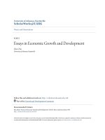
immediately following the trough. Figure 1 simply plots total nonfarm employment for the
U.S. in the post-war era. Periods of recession are shaded in gray, meaning that recoveries
begin where the shaded areas end. From this figure, we see that the post-1990 recessions
appear to differ from the typical post-war recessions in that employment does not turnaround
immediately following the start of a recovery. Rather we observe periods of continued decline
or stagnation in employment extending well beyond the end of the recession. In pre-1990
business cycles, positive growth in employment lagged the positive growth in output at the
start of a recovery by at most one quarter. In many cases, employment began its recovery
in the same quarter as output. The movement in these two series was highly correlated in
both the recession and recovery phases of the cycle. Beginning with the recovery in 1991,
we observe a change, where these two series still move together during periods of recession,
but then diverge for significant lengths of time into the recovery. (Individual plots of both
employment and output for each post-1960 recession can be found in Appendix A.)

10


140,000
130,000
120,000
110,000
100,000
90,000
80,000
70,000
60,000
50,000
40,000
1950

1955

1960

1965

1970

1975

1980

1985

1990

1995

2000

2005

2010

Figure 1: Total Nonfarm Employment (thousands). The shaded areas indicate NBER defined

recessions. Source: U.S. Bureau of Labor Statistics

As previously stated, in order to determine whether or not a given cycle contains a jobless

recovery, one must consider how the economy gains or loses jobs immediately following the
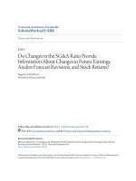
trough. Using total nonfarm payroll employment data from the Bureau of Labor Statistics
Current Employment Statistics (CES) for the post-war era, we plot the growth path of
employment around the troughs of each recession in Figure 2. We normalize employment at
the time of the trough to one for each cycle. The four series plotted are each of the three
most recent recessions and the average of the post-war recessions from 1960 up through the
1980s. Figure 2 depicts the degree to which employment continued to decline, relative to
the start of the recovery, as well as how long it took to begin adding jobs, and how long

11


it took for jobs to fully recover to their pre-recovery and pre-recession levels. From this
figure, a quick visual examination of the data shows quite clearly that the three post-1990
recessions were each accompanied by jobless recoveries. At the same time, we are able to see
how different these jobless recoveries have been from the average post-war recovery. This is
highly suggestive that these recoveries have indeed been jobless, and that jobless recoveries
may be the new norm as proposed by Schreft and Singh (2003). It should be further noted
how the jobless recoveries differ from one another when comparing the relative magnitude of
continued job loss, and the duration of joblessness. An examination of this figure may also
lead one to ask whether the condition of joblessness is a phenomenon that is worsening over
time, and if so, in what way?

12


13

Figure 2: Source: U.S. Bureau of Labor Statistics; author’s calculations
NBER defined cycle trough =1.0

0.99

1

1.01

1.02

1.03

1.04

1.05

1.06

1.07

T=average cycle, 1960-1980s
T=Nov 2001

Months from trough

T=Jun 2009
T=Mar 1991

-12
-11
-10

-9
-8
-7
-6
-5
-4
-3
-2
-1
T
1
2
3
4
5
6
7
8
9
10
11
12
13
14
15
16
17
18
19
20

21
22
23
24
25
26
27
28
29
30
31
32
33
34
35
36


3

Description of the Data

3.1

National Level

The national data for the U.S. used in this paper comes from two main sources. The national
employment data for the U.S. comes from the Bureau of Labor Statistics (BLS). The BLS
databases include data on total employment, total hours, and hours per worker, among
others, from 1947 to 2012. As a measure of total employment, the seasonally adjusted total

nonfarm employment as reported by the Current Employment Statistics (CES) survey is
used, consistent with the literature (Schreft and Singh, 2003; Aaronson, et al., 2004; Berger,
2012).
As a measure of national output, the quarterly real GDP data comes from the Bureau of
Economic Analysis (BEA). This series is in 2005 chained dollars and is seasonally adjusted.
Monthly and quarterly dates for peaks and troughs in the business cycle are taken from
the National Bureau of Economic Research (NBER) Business Cycle Dating Committee, the
accepted authority on business cycle dating. Using real GDP as the measure of output in
this paper is appropriate as it is one of the main measures of economic activity considered
by this committee in determining the dates of recessions and expansions.
For both total nonfarm employment and quarterly real GDP, analysis will only be done
including the years 1960 to 20125 . Although data for nonfarm employment and GDP are
available going back to 1947, there were significant changes made in both statistics that make
comparisons between the pre-1960 and post-1960 periods potentially problematic. Bailey
(1958) discusses how revisions made to the industrial classification system effect BLS employment statistics. He notes that, beginning in 1960, ”all national employment statistics
published by the U.S. Department of Labor’s Bureau of Labor Statistics will be revised according to a new classification system.” He continues to emphasize the potential issues by
5

Although national GDP data for 2013 became available just prior to the completion
of this draft, it was still not available at the state level. Thus, 2013 data has not been
incorporated into this draft.

14


stating, ”The extensive revision of the coding structure will have a sizable impact on the
continuity of a number of the BLS series, since the composition of many individual industries
has changed significantly.” Also, between 1947 and 1960, the BEA went through several comprehensive revisions, resulting in statistical, definitional, and presentational changes. This
presents a potential issue for both the employment and GDP series before 1960. In addition,
choosing to work only with the data beginning in 1960 or later is consistent with the extant

literature on jobless recoveries (Berger, 201; Groshen and Potter, 2003; Schreft and Singh,
2003).
Aaronson, Rissman, and Sullivan (2004) provide a very clear and detailed description of
the BLS’s two major employment surveys: the payroll survey coming from the Current Employment Statistics, and the household survey from the Current Population Survey. Both are
monthly surveys and designed to be nationally representative. Those interested in a detailed
description of the respective survey methods, the quantity of households or establishments
surveyed, what is actually being counted as employment, and the methods for extrapolating
these survey results to the whole population should refer to their paper. They detail potential flaws and biases that exist in each survey, and conclude by stating their opinion that the
payroll survey (from the Current Employment Statistics) is generally the more accurate of
the two. In addition, the majority of the existing work done in the area of jobless recoveries
has used the CES. Therefore, employment data from the CES is used throughout the paper.

3.2

State Level

State-level employment data is also taken from the BLS. Monthly total non-farm employment
data for each state is available from 1960-2012, however it is not seasonally adjusted. In order
to get a seasonally adjusted series of employment for each state over the desired sample
period, we seasonally adjust the data using the X12 ARIMA seasonal adjustment program
from the United States Census Bureau.
Recall that GDP was used as a measure of output at the national level. However, state-

15


level GDP data coming from the BEA Regional Economic Accounts and is only available
annually from 1963-2012. Annual data does not allow one to properly observe the changes
in variables throughout the business cycle. Since we need data that is at least available at a
quarterly frequency, we must find a proxy for GDP at the state level that is available at the

desired frequency.
Personal income data by state is reported on a quarterly basis by the BEA. One of
these components, called earnings by place of work, was chosen as our proxy of state output.
According to the BEA, ”Earnings by place of work is the sum of Wage and Salary Disbursements, supplements to wages and salaries and proprietor’s income. BEA presents earnings
by place of work because it can be used in the analysis of regional economies as a proxy for
the income that is generated from participation in current production.” Thus, we feel that
earnings by place of work has the potential to be a reasonably strong proxy for state output.
Henceforth, earnings by place of work will be referred to as simply earnings for short.
Additional adjustments must be made to the earnings data to make the series more
comparable to the measure of output used at the national level (GDP), and to allow for
meaningful comparison across time and states. The earnings data is nominal and not seasonally adjusted. We first seasonally adjust the earnings data for each state using the X12
ARIMA process discussed above. The nominal, seasonally adjusted series is then converted
into real earnings using the GDP deflator. This provides a real, seasonally adjusted earnings
measure for each state which can be used as a proxy for output.
Other proxies for output face challenges either in the frequency or range of the available
data. For instance, GDP by state is available over the desired range, but only at an annual
frequency. Data on commercial electricity consumption by state, which is believed to be
highly correlated with production, is avaiable monthly, but only as far back as 1990. Since
both of these alternative proxies have their shortcomings in the context of this particular
study, they cannot be used here.
The data seem to support the claim of the BEA that earnings by place of work may

16


proxy well for production. The average correlation coefficient between annual state GDP
levels and annual state earnings by place of work is 0.9977. Thus, at the state level, the
correlation between GDP and our proxy seems very strong when using the annual data. Of
course, we cannot evaluate whether this is also true when using quarterly data (quarterly,
state-level GDP measures do not exist); but we still made an effort to document the quarterly

correlation at the national level. National data for both GDP and earnings by place of work
are available at a quarterly frequency and have a correlation of 0.7272. Both the annual
state-level correlations and the quarterly national-level correlations suggest that earnings is
indeed a reasonable proxy for GDP.
In addition, given that for the purpose of calculating the JRD we require an approximation for the percentage changes in GDP and not for the GDP levels themselves, we also
looked at how annual changes in earnings at the state level correlate with annual changes
in state-level GDP. We conducted standard OLS regressions between the state-level, annual
changes in GDP and the corresponding state-level annual changes in earnings. In these regressions, earnings are significant at the 1% level for all 50 states and explain about 75.6%
of the observed variation in GDP, on average (the average R-squared for the 50 regressions
was 0.756).

4
4.1

The Jobless Recovery Depth and Other Measures of Jobless Recoveries

Unsophisticated Measures of Duration

Although evidence has been provided on the existence of jobless recoveries, there has been
little to no attempt made to measure them in a meaningful way. Questions regarding the
severity of a jobless period and whether there is a discernible trend or pattern over time are
difficult to answer without meaningful measures. Using the definition of a jobless recovery
from Schreft and Singh (2003), recall that a recovery is considered to be jobless “if the
growth rate of employment in a recovery is not positive.” This definition is consistent with
the related literature. We begin by constructing a simple measure out of this definition:
17


merely counting the number of months or quarters that a given recovery was jobless. This is
accomplished by calculating the number of quarters or months where positive output growth

was accompanied by nonpositive employment growth, once again using the NBER defined
cycle troughs as the start of a recovery. This is reported in Figure 3 using national data.
The results from counting the number of jobless quarters are redundant, so only monthly
measures are reported here.
This simple definition we have taken from the literature for a jobless recovery generates
nothing more than a simple indicator variable. At any given point in time, a recovery is
either jobless, or it’s not; a 1, or a 0. The issue with creating a binary variable to use
in our analysis of jobless recoveries is that, apart from duration, it tells us nothing about
how these jobless periods have differed from one another. (It should be noted that the
simple measure of duration this provides is alone an improvement over the previous research
on jobless recoveries). Comparing a 1 to a 1 in different business cycles suggests these
jobless periods are the same. Does it seem likely that all periods of time defined as jobless
are equal? The data clearly suggest otherwise, yet with this simple indicator variable, we
glean no additional information. This simple classification neglects important details in the
movements of these variables over time. One example is that it fails to account for the
relative magnitude of job losses and gains. In fact, the losses to total employment incurred
over the jobless period following a recover may not be regained for many months or even
years. This may be accompanied by strong or weak growth in aggregate output, and the
weakness of the labor market relative to output growth is lost on a binary variable. Apart
from producing the simple measures of duration reported in Figure 3, this indicator variable
for jobless recoveries can tell us little else. Yet there has been no previous attempt made to
move away from so restrictive a definition of jobless recoveries.

18


Figure 3: Unsophisticated measures of duration using monthly data

19

0

5

10

15

20

25

30

35

40

45

50

1991

months to return to pre-recession employment

Months without employment growth (standard)

avg 1960-1990

Months to return to pre-recovery employment

2001

2007


For example, in the recovery following the Great Recession, there were only three jobless
quarters according to this aforementioned definition. However, it took eight quarters for
employment to regain its pre-recovery level. Meaning that two years after output began to
recover; jobs had experienced zero net growth relative to the start of said recovery. Could one
not also argue then that this whole period of time could be considered jobless? We see that
the determination of how long joblessness lasts during a recovery depends very strongly on
the interval of time being considered. If instead of using quarterly data, one used annual or
monthly data as the interval of time, one might find that relatively longer or shorter periods
fall under the jobless recovery label currently being used in the literature. Thus, measuring
the length of time it takes for employment to reach a positive net gain relative to the start
of the recovery may be an informative measure for joblessness as well. This measure is also
presented in Figure 3. Moreover, we feel it is meaningful to quantify the length of time
it takes for total employment to return to its pre-recession peak, in other words, how long
it takes for employment to make a full recovery. This count is also presented in Figure 3.
Inspecting Figure 3, we see that according to all of these measures the post-1990 recoveries
have been jobless. Additionally, we see that most of these measures suggest a trend towards
recoveries with an increasingly long duration of joblessness over time. This provides further
evidence of a change in the economy away from the historical relationship between output
and labor.

4.2

The Relative Job Loss

Although meaningful, these simple counting measures offer only a glimpse of what can be
gained from quantifiably measuring jobless recoveries. We now propose a new measure
of employment during the business cycle that should be much more informative. In the
macroeconomic and econometrics literatures, there is a useful measure for gauging the depth
of a recession at any point in time known as the Current Depth of Recession (CDR). CDR
was first proposed by Beaudry and Koop (1993). CDR is defined as the gap between the
20