Spatial analysis of soil chemical properties of Bastar district, Chhattisgarh, India

Int.J.Curr.Microbiol.App.Sci (2019) 8(4): 2185-2197

International Journal of Current Microbiology and Applied Sciences
ISSN: 2319-7706 Volume 8 Number 04 (2019)
Journal homepage:

Original Research Article

/>
Spatial Analysis of Soil Chemical Properties of Bastar District,
Chhattisgarh, India
P. Smriti Rao1*, Tarence Thomas1, Amit Chattree2,
Joy Dawson3 and Narendra Swaroop1
1

Department of Soil Science, 2Department of Chemistry, 3Department of Agronomy,
Sam Higginbottom University of Agriculture, Technology & Sciences- 211007 Allahabad,
U.P., India
*Corresponding author

ABSTRACT

Keywords
Geostatistics,
Coefficient of
variance, Ordinary
kriging, etc.

Article Info
Accepted:
17 March 2019

Available Online:
10 April 2019

Mapping of soil properties is an important operation as it plays an important role in the
knowledge about soil properties and how it can be used sustainably. The study was carried
out in a Bastar district, Chhattisgarh state, India in order to map out some soil
characteristics and assess their variability within the area. Samples were collected from the
4 sampling sites, Kesloor and Raikot (NH-16), Adawal and Nagarnar (NH-43) in
Jagdalpur. From each site, 6 samples of soils (with three replications) from 20m, 60m and
500m (control site) distance from the edge of national highway at two soil depths, 0-20
cm, and 20-40 cm were collected respectively. The soil samples were air-dried, crushed
and passed through a 2 mm sieve before analyzing it for pH, EC, Organic carbon, Iron,
Copper and Lead were calculated. After the normalization of data classical statistics was
used to describe the soil properties and geo-statistical analysis was used to illustrate the
spatial variability of the soil properties by using kriging interpolation techniques in a GIS
environment. Results showed that the coefficient of variance for all the variables was 2.33
to 2.42 at depth 0-20cm and 2.34 to 2.41 at depth 20-40 cm. The geostatistical analysis
was done by Ordinary kriging.

Introduction
Soil is a dynamic natural body which
develops as a result of pedogenic natural
processes during and after weathering of
rocks. It consists of mineral and organic
constituents, processing definite chemical,
physical, mineralogical and biological
properties having a variable depth over the
surface of the earth and providing a medium
for plant growth (Biswas and Mukherjee,

1994). Soil is a heterogeneous, diverse and
dynamic system and its properties change in
time and space continuously (Rogerio et al.,
2006). Heterogeneity may occur at a large
scale (region) or at small scale (community),
even in the same type of soil or in the same
community (Du Feng et al., 2008). Soil which
is a natural resource has variability inherent to
how the soil formation factors interact within
the landscape. However, variability can occur
also as a result of cultivation, land use and

2185


Int.J.Curr.Microbiol.App.Sci (2019) 8(4): 2185-2197

erosion. Salviano (1996) reported spatial
variability in soil attributes as a result of land
degradation due to erosion. Spatial variability
of soil properties has been long known to
exist and has to be taken into account every
time field sampling is performed and
investigation of its temporal and spatial
changes is essential.
Geographical information system (GIS)
technologies has great potentials in the field
of soil and has opened newer possibilities of
improving soil statistic system as it offers
accelerated, repetitive, spatial and temporal

synoptic view. It also provides a cost effective
and accurate alternative to understanding
landscape dynamics. GIS is a potential tool
for handling voluminous data and has the
capability to support spatial statistical
analysis, thus there is a great scope to
improve the accuracy of soil survey through
the application of GIS technologies.
Therefore, assessing spatial variability
distribution on nutrients in relation to site
characteristics including climate, land use,
landscape position and other variables is
critical for predicting rates of ecosystem
processes
(Schimel
et
al.,
1991),
understanding
how
ecosystem
work
(Townsend et al., 1995) and assessing the
effects of future land use change on nutrients
(Kosmas et al., 2000).
Out of the 118 elements in nature about 80 are
metals, most of which are found only in trace
amounts in the biosphere and in biological
materials. There are at least some twenty
metals like elements which give rise to well

organize toxic effects in man and his
ecological associates. Metals having density
of more than 6mg/m3 and atomic weight more
than iron are called has heavy metals. Some
metals and material and metalloids such as
Zinc (Zn), copper (Cu), manganese (Mn),
Nickel (Ni), cobalt (Co), chromium (Cr)
molybdenum (Mb), and iron (Fe) are the

essential are essential for living organisms.
The contamination from automobiles are
accumulated on the soil surface, move down
to deep layers of soil and eventually change
the soil physio-chemical properties directly or
indirectly metals contamination in soil ranges
from less than 1 ppm to as high as 100,000
ppm due to human activity. The roadside
environment represents a complex system for
heavy metals in term of accumulation
transport pathways and removal processes
(Ghosh et al., 2003). Therefore, learning of
the extent of heavy metals contamination on
highway sites and its inflow into plant is
highly relevant to the management of
sustainable urban environmental quality
everywhere. Study of the heavy metals
contamination on highway sights soil and its
accumulation highway side plant is highly
relevant in India because of high urban
development associated with an exponential

rise in the number of vehicles on the
highways having no effective pollution
control standards.
Out of 4 study areas 2 are situated near the
National mineral development corporation
and 2 villages at different direction from it.
The influence of the development of NMDC
on the soil physicochemical characteristics is
the primary objective of the study. Soil is a
dynamic natural body which develops as a
result of pedogenic natural processes during
and after weathering of rocks. It consists of
mineral and organic constituents, processing
definite chemical, physical, mineralogical and
biological properties having a variable depth
over the surface of the earth and providing a
medium for plant growth (Biswas and
Mukherjee, 1994). Soil is a heterogeneous,
diverse and dynamic system and its properties
change in time and space continuously
(Rogerio et al., 2006). Heterogeneity may
occur at a large scale (region) or at small scale
(community), even in the same type of soil or

2186


Int.J.Curr.Microbiol.App.Sci (2019) 8(4): 2185-2197

in the same community (Du Feng et al.,

2008). Soil which is a natural resource has
variability inherent to how the soil formation
factors interact within the landscape.
However, variability can occur also as a result
of cultivation, land use and erosion. Salviano
(1996) reported spatial variability in soil
attributes as a result of land degradation due
to erosion. Spatial variability of soil
properties has been long known to exist and
has to be taken into account every time field
sampling is performed and investigation of its
temporal and spatial changes is essential.
Geographical information system (GIS)
technologies has great potentials in the field
of soil and has opened newer possibilities of
improving soil statistic system as it offers
accelerated, repetitive, spatial and temporal
synoptic view. It also provides a cost effective
and accurate alternative to understanding
landscape dynamics. GIS is a potential tool
for handling voluminous data and has the
capability to support spatial statistical
analysis, thus there is a great scope to
improve the accuracy of soil survey through
the application of GIS technologies.
Therefore, assessing spatial variability
distribution on nutrients in relation to site
characteristics including climate, land use,
landscape position and other variables is
critical for predicting rates of ecosystem

processes
(Schimel
et
al.,
1991),
understanding
how
ecosystem
work
(Townsend et al., 1995) and assessing the
effects of future land use change on nutrients
(Kosmas et al., 2000). Out of the 118
elements in nature about 80 are metals, most
of which are found only in trace amounts in
the biosphere and in biological materials.
There are at least some twenty metals like
elements which give rise to well organize
toxic effects in man and his ecological
associates. Metals having density of more
than 6mg/m3 and atomic weight more than
iron are called has heavy metals. Some metals
and material and metalloids such as Zinc

(Zn), copper (Cu),manganese (Mn), Nickel
(Ni),
cobalt
(Co),
chromium
(Cr)
molybdenum (Mb), and iron (Fe) are the

essential are essential for living organisms.
The contamination from automobiles are
accumulated on the soil surface, move down
to deep layers of soil and eventually change
the soil physio-chemical properties directly or
indirectly metals contamination in soil ranges
from less than 1 ppm to as high as 100,000
ppm due to human activity. The roadside
environment represents a complex system for
heavy metals in term of accumulation
transport pathways and removal processes
(Ghosh et al., 2003). Therefore, learning of
the extent of heavy metals contamination on
highway sites and its inflow into plant is
highly relevant to the management of
sustainable urban environmental quality
everywhere. Study of the heavy metals
contamination on highway sights soil and its
accumulation highway side plant is highly
relevant in India because of high urban
development associated with an exponential
rise in the number of vehicles on the
highways having no effective pollution
control standards. Out of 4 study areas 2 are
situated
near
the
National
mineral
development corporation and 2 villages at

different direction from it. The influence of
the development of NMDC on the soil
physicochemical characteristics is the primary
objective of the study.
Materials and Methods
Study area
The study was carried out in Bastar district,
Chattisgarh state, India (Fig. 1). It has its
headquarters in the town of Jagdalpur.
Jagdalpur has a monsoon type of hot tropical
climate. Summers last from March to May
and are hot, with the average maximum for
May reaching 38.1 °C (100.6 °F). The
weather cools off somewhat for the monsoon

2187


Int.J.Curr.Microbiol.App.Sci (2019) 8(4): 2185-2197

season from June to September, which
features very heavy rainfall. Winters are
warm and dry. Its average rainfall is 1324.3
mm. Its average temperature in summer is
33.15°C, and in winter is 20.73°C. Samples
were collected from the 4 sampling sites,
Kesloor and Raikot (NH-16), Adawal and
Nagarnar (NH-43) in Jagdalpur. From each
sites, 6 samples of soils (with three
replications) from 20m, 60m and 500m

(control site) distance from the edge of
national highway at two soil depths, 0-20 cm,
and 20-40 cm were collected. The soil
samples were transferred in to air tight
polythene bags and will be brought to the PG
laboratory of Deptt. Of Soil Science and
Agricultural Chemistry, SHUATS, Allahabad.

technique within the spatial analyst extension
module in ArcGis 10.2 software package to
determine the spatial dependency and spatial
variability of soil properties. Kriging method
is a statistical estimator that gives statistical
weight to each observation so their linear
structure’s has been unbiased and has
minimum estimation variance (Kumke et al.,
2005). This estimator has high application due
to minimizing of error variance with unbiased
estimation
(Pohlmann,
1993).
The
experimental
variogram
model
was
constructed using the Kriging method, with
data obtained from the research area. The
spatial transformation was performed to
determine the most appropriate model to use

with the parameters of the generated maps.

Soil analysis

The ordinary Kriging formula is as follows:
(Isaaks and Srivastava, 1989; ESRİ, 2003).

The soil samples were air-dried, crushed and
passed through a 2 mm sieve. Soil samples
were analyzed for soil pH in both water and
0.01 M potassium chloride solution (1:1)
using glass electrode pH meter (McLean,
1982). EC was determined by using Digital
Electrical conductivity method. Soil organic
carbon was estimated by Walkley and Black
method. Soil Iron, Copper and Lead was
analysed by Wet digestion method, taking
Aqua regia (1:3 HNO3:HCl) for digestion and
finding the results through AAS (Perkin
Elmer A Analyst).
Statistical analysis
Statistical analysis for the work was done in
two stages. Firstly, the distribution of data
was described using conventional statistics
such as mean, median, minimum, maximum,
standard deviation (SD), skewness and
kurtosis in order to recognize how data is
distributed and each soil characteristics were
investigated using descriptive statistics.
Secondly, geo-statistical analysis was

performed using the kriging interpolation

where Z(Si) is the measured value at the
location (ith), λi is the unknown weight for
the measured value at the location (ith) and S0
is the estimation location. The unknown
weight (λp) depends on the distance to the
location of the prediction and the spatial
relationships among the measured values.
The statistical model estimates the
unmeasured values using known values. A
small difference occurs between the true
value Z(S0) and the predicted value, Σ_iZ(Si).
Therefore, the statistical prediction is
minimized using the following formula:

The Kriging interpolation technique is made
possible by transferring data into the GIS
environment. In this way, analysis in areas
that have no data can be conducted. The
following criteria were used to evaluate the
model: the average error (ME) must be close

2188


Int.J.Curr.Microbiol.App.Sci (2019) 8(4): 2185-2197

to 0 and the square root of the estimated error
of the mean standardized (RMSS) must be

close to 1 (Johnston et al., 2001). While
implementing the models, the anisotropy
effect was surveyed.

ground water and irrigation water quality
(Abel et al., 2014; Al-Atab, 2008; Al-Juboory
et al., 1990).

Results and Discussion

The possible spatial structure of the different
soil properties were identified by calculating
the semivariograms and the best model that
describes these spatial structures was
identified. These results are shown in Tables
4 and 5 for the two depths. The model with
the best fit was applied to each parameter, the
Exponential and Gaussian model was the best
fit for all parameters. The nugget effect (Co),
the sill (Co + C) and the range of influence
for each of the parameters were noted. The
spatial dependencies (Nugget/Sill ratio) were
found to be related to the degree of
autocorrelation between the sampling points
and expressed in percentages. Table 4 shows
the
soil
properties
where
variable

characteristics
were
generated
from
semivariogram model. C0 is the nugget
variance; C is the structural variance, and C0
+ C represents the degree of spatial
variability, which affected by both structural
and stochastic factors (Fig. 2 and 3). The
higher ratio indicates that the spatial
variability is primarily caused by stochastic
factors, such as fertilization, farming
measures, cropping systems and other human
activities. The lower ratio suggests that
structural factors, such as climate, parent
material, topography, soil properties and other
natural factors, play a significant role in
spatial variability. The spatial dependent
variables was classified as strongly spatially
dependent if the ratio was <25, moderately
spatially dependent if the ratio is between 25
and 75% while it is classified as weak spatial
dependent if it >75% (Cambardella et al.,
1994; Clark, 1979; Erşahin, 1999; Robertson,
1987; Trangmar et al., 1985).
For the 0–20 cm depth, Ph, EC, %OC, Fe, Ni
and Cr had a strong spatial dependence with a

Soil mapping and survey is an important
activity because it plays a key role in the

assessment of soil properties and its use in
agriculture, irrigation and other land uses.
This study was carried out to assess the
spatial variability of some physical and
chemical soil properties so as to determine
their current situations in the study area,
therefore the results can be presented as
follows:
Descriptive statistics
The summary of the descriptive statistics of
soil parameters as shown in Table 1 suggest
that they were all normally distributed. The
coefficient of variance for all the variables
was 2.33 to 2.42 at depth 0-20cm and 2.34 to
2.41 at depth 20-40 cm. All the variables
show low variation according to Coefficient
of variance according to the guidelines
provided by Warrick, 1998 for the variability
of soil properties. The lowest coefficient of
variation could be as a result of the uniform
conditions in the area such as little changes in
slope and its direction leading to a uniformity
of soil in the area (Afshar et al., 2009;
Cambardella et al., 1994; Kamare, 2010).
Most of the soil properties were highly
positively skew at both depths i.e. pH and EC
at Raikot, Kesllor and Chokawada while
%OC, Fe, Ni and Cr were both symmetrical.
These variations in chemical properties are
mostly related to the different soil

management practices carried out in the study
area,
the
vehicle
transportation,
environmental pollution, parent material on
which the soil is formed, role of the depth of

Geostatistical analysis

2189


Int.J.Curr.Microbiol.App.Sci (2019) 8(4): 2185-2197

ratio of 0.28, 0, 0.99, 0, 0, and 0%
respectively (Table 4).
At the lower depth i.e. 20–40 cm pH, EC,
%OC, Fe, Ni and Cr had a strong spatial
dependence (0.214, 0, 0.99, 0.475, 0 and
0.121%) (Table 4 and Fig. 4–9).

samples have similar and different values
respectively. Therefore, nugget effects that is
small and close to zero indicates a spatial
continuity between the neighboring points,
this can be backed with the results of Vieira
and Paz Gonzalez (2003) and Mohammad
Zamani et al., (2007).

The value of nugget effect for EC, Fe and Ni
were the lowest at both depths which suggest
that the random variance of variables is low in
the study area, this implies that near and away

The presence of a sill on the variogram
indicates second-order stationarity, i.e. the
variance and covariance exist (Table 2)
(Geoff Bohling, 2005).

Table.1 Descriptive statistics within the field grid for the variables at depth 0-20 cm
Village Raikot (Distance fromNH at 20 m, 60 m and 500m)
pH
EC
%OC
Fe
Ni
Statistics
6.30667
.42367
.89667
1585.00000
Mean
6.25000
.40300
.91000
2088.00000
Median
.162583
.043822

.080829
907.837541
SD
1.378
1.650
-.722
-1.728
Skewness
Village Kesloor (Distance fromNH at 20 m, 60 m and 500m)
6.62333
.48233
.88333
2174.00000
Mean
6.60000
.45700
.88000
2176.00000
Median
.040415
.145662
.015275
37.040518
SD
1.732
.759
.935
-.242
Skewness
Village Adawal (Distance fromNH at 20 m, 60 m and 500m)

7.06000
.56033
1.07667
2287.33333
Mean
7.07000
.55900
1.06000
2355.00000
Median
.017321
.089007
.037859
135.795189
SD
-1.732
.067
1.597
-1.686
Skewness
Village Chokawada (Distance fromNH at 20 m, 60 m and 500m)
6.87667
.46133
.92333
2279.66667
Mean
6.96000
.46800
.92000
2280.00000

Median
.153080
.042395
.025166
.577350
SD
-1.724
-.690
.586
-1.732
Skewness

2190

Cr
6.13333

6.33333

7.50000

5.00000

3.647373

3.028751

-1.449

1.597

12.93333

16.73333

13.50000

15.30000

4.675824

2.569695

-.537

1.729

15.40000

25.33333

13.50000

20.80000

4.838388

10.279267

1.495

1.599

17.20000

41.43333

16.90000

26.90000

2.662705

25.868385

.501

1.730


Int.J.Curr.Microbiol.App.Sci (2019) 8(4): 2185-2197

Table.2 Descriptive statistics within the field grid for the variables at depth 20-40 cm
Village Raikot (Distance from NH at 20 m, 60 m and 500m)
pH
EC
%OC
Fe
Statistics
6.23333

.44033
.74333
1057.00000
Mean
6.21000
.42700
.75000
1367.00000
Median
.116762
.050342
.050332
621.027375
SD
.863
1.108
-.586
-1.687
Skewness
Village Kesloor (Distance from NH at 20 m, 60 m and 500m)
6.61333
.51867
.74000
2081.33333
Mean
6.60000
.46200
.74000
2091.00000
Median

.023094
.161630
.020000
21.221059
SD
1.732
1.384
.000
-1.625
Skewness
Village Adawal (Distance from NH at 20 m, 60 m and 500m)
7.00000
.63933
.90667
2060.33333
Mean
7.06000
.64100
.92000
2087.00000
Median
.112694
.047522
.032146
151.767366
SD
-1.717
-.158
-1.545
-.766

Skewness
Village Chokawada (Distance from NH at 20 m, 60 m and 500m)
6.76667
.48933
.73333
2305.33333
Mean
6.71000
.50200
.72000
2354.00000
Median
.191398
.055103
.041633
84.293139
SD
1.216
-.980
1.293
-1.732
Skewness

Ni

Cr

4.03333

1.16667

2.90000

.00000

3.635015

2.020726

1.267

1.732

11.83333

11.76667

11.10000

10.10000

4.247744

5.012318

.754

1.331

12.53333

16.26667

10.70000

15.90000

3.980368

1.582193

1.633

.987

30.46667

33.26667

26.40000

35.40000

17.948909

7.433259

.967

-1.185

Table.3 Coefficient of variation within the field grid at depth 0-20 cm and 20-40 cm
Area
R 20 m
R 60 m
R 500 m
K 20 m
K 60 m
K 500 m
A 20 m
A 40 m
A 500 m
C 20 m
C 60 m
C 500 m

Cov (Depth 0-20 cm)
2.41
2.42
2.37
2.39
2.4
2.41
2.36
2.4
2.4
2.33
2.38
2.39

2191

Cov (Depth 20-40cm)
2.41
2.43
2.38
2.39
2.41
2.41
2.39
2.39
2.4
2.36
2.39
2.34


Int.J.Curr.Microbiol.App.Sci (2019) 8(4): 2185-2197

Table.4 Geostatistical parameters of the fitted semivariogram models for soil properties and
cross validation statistics at 0-20 cm depth and 20-40 cm depth respectively
Variable
pH

Nugget
(C0)
0.0069

Sill
(C0+C)

0.241

EC

0

0.0109

OC

3.81

3.825

Fe

0

Cu
Pb
Variable
pH
EC
OC
Fe
Ni
Cr

230769.
6

0
22.40
181.26
0
Nugget( Sill
C0)
(C0+C)
0.030
0.11
0
0.016
1.30
1.313
211036. 444118.
30
8
0
194.33
34.64
286.12

Rang
e (A)
0.353
4
0.138
6
0.170
1
0.138

Nugget/
Sill
0.28

Model

RMS

ME

Exponential

Spatial
Class
strong

0.152

0.038

0

Exponential

strong

0.099

0.0389

0.99

Exponential

strong

0.058

0.255

0

Exponential

strong

515.79

0.057

0.138
0.353
Rang
e (A)
0.252
0.132
0.16
0.353

0
0
Nugget/
Sill
0.215
0
0.99
0.475

Exponential
Exponential
Model

4.046
15.22
RMS

0.049
0.044
ME

Exponential
Exponential
Gaussian
Exponential

strong
Strong
Spatial
Class

Strong
Strong
Strong
Strong

0.207
0.121
0.080
535.15

0.016
0.060
0.120
0.027

0.132
0.353

0
0.121

Exponential
Exponential

strong
strong

12.69
7.85

0.057
0.016

Fig.1 Map of the study area of Bastar district, Chhattisgarh, India showing the sample locations

2192


Int.J.Curr.Microbiol.App.Sci (2019) 8(4): 2185-2197

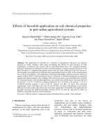
Fig.2 Semivariogram parameters of best fitted theoretical model to predict soil properties at 0-20
cm depth, a. pH b. EC c. %OC d. Fe e. Cu and f. Pb

(a)

(b)

(d)

(e)

(c)

(f)

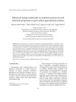
Fig.3 Semivariogram parameters of best fitted theoretical model to predict soil properties at 2040 cm depth, a. pH b. EC c. %OC d. Fe e. Ni and f. Cr

(a)

(d)

(b)

(c)

(e)
2193

(f)


Int.J.Curr.Microbiol.App.Sci (2019) 8(4): 2185-2197

Fig.4 (a) pH at 0-20cm and (b) pH at 20-40cm

(a)

(b)

Fig.5 (a) EC at 0-20cm and (b) EC at 20-40cm

(a)

(b)

Fig.6 (a) OC at 0-20cm and (b) OC at 20-40cm

(a)

(b)

Fig.7 (a) Fe at 0-20cm and (b) Fe at 20-40cm

(a)

(b)
2194


Int.J.Curr.Microbiol.App.Sci (2019) 8(4): 2185-2197

Fig.8 (a) Ni at 0-20cm and (b) Ni at 20-40cm

(a)

(b)
Fig.9 (a) Cr at 0-20cm and (b) Cr at 20-40cm

(a)

(b)

In conclusion, assessing spatial variability and
mapping of soil properties is an important
pre-requisite for soil and crop management
and also useful in identifying land
degradation spots. The production of soil
nutrient maps is the first step in precision
agriculture because these maps will measure
spatial variability and provide the basis for
controlling it. It would also help in reducing

the amount of inputs been added to the soil in
form of supplements so as not to over burden
the soil which can lead to pollution thereby
degrading the land. The results shows that the
spatial distribution and spatial dependence
level of soil properties can be different even
within the same local government area. It also
demonstrates the effectiveness of GIS
techniques in the interpretation of data. These
results can be used to make recommendations
of best management practices within the
locality and also to improve the livelihood of
smallholder farmers.

References
Abel, C., Kutywayo, D., Chagwesha, T. M.,
and Chidoko, P. (2014). Assessment of
irrigation water quality and selected soil
parameters at Mutema irrigation
scheme, Zimbabwe. Journal of Water
Resources and Protection, 6, 132–140.
Afshar, H., Salehi, M. H., Mohammadi, J.,
and Mehnatkesh, A. (2009). Spatial
variability of soil properties and
irrigated wheat yield in quantitative
suitability map, a case study: Share e
Kian Area, Chaharmahaleva Bakhtiari
province. Journal of Water and Soil, 23,
161–172.
Al-Atab, S. M. S. (2008). Variations of soil

properties and classification in some
area of Basrah Governorate (PhD
Thesis). College of Agriculture,
University of Basrah, Basrah.
Al-Juboory, S. R., Alaqid, W. K. Alaqidi and

2195


Int.J.Curr.Microbiol.App.Sci (2019) 8(4): 2185-2197

Al-Issawi, S. M. (1990). Effect of soil
management practices on Chemical and
physical properties of a soil from great
Mussayb Project. Iraqi journal of
Agriculture Sciences, 21, 107–116.
Biswas, T. D., and Mukherjee, S. K. (1994).
Textbook of soil science. New Delhi:
Tata McGraw-Hill Publishing Company
Limited.
Black, C. A. (1965). Methods of soil analysis.
Agronomy No. 9, Part 2. Madison, WI:
American Society of Agronomy.
Brown, G., Newman, A. C. D., Rayner, J. H.,
Weir, A. H. (1978). The structure and
chemistry of soil clay minerals In D. J.
Greenland and M. H. B. Hayes (Eds.),
The chemistry of soil constituents(pp.
29178). New York, NY: Wiley.
Buol, S. W., Hole, F. D., McCracken, R. J.,

and Southard, R. J. (1997). Soil genesis
and classification (4th ed., p. 527).
Ames: Iowa State University Press.
Cambardella, C. A., and Karlen, D. L. (1999).
Spatial analysis of soil fertility
parameters. Precision Agriculture, 1, 5–
14.
Cambardella, C. A., Moorman, T. B., Parkin,
T. B., Karlen, D. L., Novak, J. M.,
Turco, R. F., and Konopka, A. E.
(1994). Field-scale variability of soil
properties in central Iowa soils. Soil
Science Society of America Journal, 58,
1501–1511.
http://
dx.doi.org/10.2136/sssaj1994.03615995
005800050033x
Clark, I. (1979). Practical geostatistics (p.
129). London: Applied Science
Publishers.
Du Feng, L. Z., XuXuexuan, Z. X., and Shan,
L. (2008). Spatial heterogeneity of soil
nutrients and aboveground biomass in
abandoned old-fields of Loess Hilly
region in Northern Shaanxi, China. Acta
Ecologica Sinica, 28, 13–22.
Erşahin, S. (1999). Alluvial soil in a field,
some physical and chemical properties

of the spatial variability of the

determination. SU Journal of the
Faculty of Agriculture, 13, 34–41.
ESRİ. (2003). The principles of geostatistical
analysis (p. 54). Federal Fertilizer
Department. Federal Ministry of
Agriculture and Rural development.
(2012). Fertilizer use and management
practices for crops in Nigeria (4th ed.,
pp. 40–41).
Isaaks, E. H., and Srivastava, R. M. (1989).
An introduction to applied geostatistics.
New York, NY: Oxford University
Press.
Jackson M. L. (1958). Soil chemical analysis
(p. 125). Engle wood cliffs, NJ: Prentice
Hall.
Johnston, K., Hoef, M., Krivoruchko, K., and
Lucas, N. (2001). Using ArcGIS
geostatistical analyst. New York, NY:
ESRI.
Kamare, R. (2010). Spatial variability of
production, density and canopy cover
percentage of Nitrariaschoberi L. in
Meyghan Playa of Arak by using
geostatistical methods (M.Sc Thesis,
76pp). Tarbiat Modares University, Tehran.
Kosmas, C., Gerontidis, St., and Marathianou,
M. (2000). The effect of land use
change on soils and vegetation over
various lithological formations on

Lesvos (Greece). Cantena, 40, 51–68.
Kumke, T., Schoonderwaldt, A., and Kienel,
U. (2005). Spatial variability of
sedimentological properties in a large
Siberian lake. Aquatic Sciences, 67, 86–
96. />López-Granados, F., Jurado-Expósito, M.,
Atenciano, S., García- Ferrer, A.,
Sánchez de la Orden, M. S., and GarcíaTorres, L. (2002). Spatial variability of
agricultural soil parameters in southern
Spain. Plant and Soil, 246, 97–105.
/>5380

2196


Int.J.Curr.Microbiol.App.Sci (2019) 8(4): 2185-2197

McLean, E. O. (1982). Soil pH and lime
requirement. In A. L. Page (Ed.),
Methods of soil analysis part 2.
Madison, WI: ASA-SSSA.
Mohammad Zamani, S., Auubi, S., and
Khormali, F. (2007). Investigation of
spatial variability soil properties and
wheat production in some of farmland
of sorkhkalateh of Golestan province.
Journal of Science and Technical
Agriculture and Natural Recourses, 11,
79–91.
Pohlmann,

H.
(1993).
Geostatistical
modelling of environmental data.
CATENA,
20,
191–198.
/>
8162(93)90038-Q
Robertson, G. P. (1987). Geostatistics in
ecology: Interpolating with known
variance. Ecology, 68, 744–748.
/>Rogerio, C., Ana, L. B. H., and de Quirijn, J.
L. (2006). Spatiotemporal variability of
soil water tension in a tropical soil in
Brazil. Geoderma, 133, 231–243.
Salviano, A. A. C. (1996). Variabilidade de
atributos de solo e crotalária júncea em
solo degradado do município de
Piracicaba – SP (p. 91). Piracicaba:
Tese (Doutorado), Escola Superior de
Agricultura
Luiz
de
Queiroz,
Universidade de São Paulo.

How to cite this article:
Smriti Rao, P., Tarence Thomas, Amit Chattree, Joy Dawson and Narendra Swaroop. 2019.
Spatial Analysis of Soil Chemical Properties of Bastar District, Chhattisgarh, India.

Int.J.Curr.Microbiol.App.Sci. 8(04): 2185-2197. doi: />
2197