No small hairs in anisotropic power law Gauss-Bonnet inflation
Bạn đang xem bản rút gọn của tài liệu. Xem và tải ngay bản đầy đủ của tài liệu tại đây (230.31 KB, 15 trang )
Communications in Physics, Vol. 29, No. 2 (2019), pp. 173-187
DOI:10.15625/0868-3166/29/2/13677
NO SMALL HAIRS IN ANISOTROPIC POWER-LAW GAUSS-BONNET
INFLATION
TUAN Q. DO † AND SONNET HUNG Q. NGUYEN
Faculty of Physics, VNU University of Science,
Vietnam National University, Hanoi 120000, Vietnam
† E-mail:
Received 11 March 2019
Accepted for publication 2 May 2019
Published 15 May 2019
Abstract. We will examine whether anisotropic hairs exist in a string-inspired scalar-GaussBonnet gravity model with the absence of potential of scalar field during the inflationary phase.
As a result, we are able to obtain the Bianchi type I power-law solution to this model under the
assumption that the scalar field acts as the phantom field, whose kinetic is negative definite. However, the obtained anisotropic hair of this model turns out to be large, which is inconsistent with
the observational data. We will therefore introduce a nontrivial coupling between scalar and vector fields such as f 2 (φ )Fµν F µν into the scalar-Gauss-Bonnet model with the expectation that the
anisotropic hair would be reduced to a small one. Unfortunately, the magnitude of the obtained
anisotropic hair is still large. These results indicate that the scalar-Gauss-Bonnet gravity model
with the absence of potential of scalar field might not be suitable to generate small anisotropic
hairs during the inflationary phase.
Keywords: Gauss-Bonnet gravity, Inflation, Bianchi type I metric, Cosmic no-hair conjecture.
Classification numbers: 98.80.-k, 98.80.Cq, 98.80.Jk.
I. INTRODUCTION
In cosmology, the Copernican principle, which states without any proofs that any spacetime
describing the whole universe is just simply homogeneous and isotropic, has played a central
role. According to this principle, the homogeneity and isotropy of universe should remain over
its timeline. Testing the validity of the Copernican principle has been indeed a very important but
not straightforward task for physicists and cosmologists [1]. Along with this principle, the has
c 2019 Vietnam Academy of Science and Technology
174
TUAN Q. DO AND SONNET HUNG Q. NGUYEN
existed the so-called cosmic no-hair conjecture proposed by Hawking and his colleagues is also
concerning the property of spacetime of universe [2]. In particular, this conjecture claims that a
final state of our universe should be homogeneous and isotropic, regardless of any inhomogeneous
and/or anisotropic initial states. This conjecture seems to be more general than the Copernican
principle since it regards the evolution of universe from the past to the future. Unfortunately, a
complete proof for this conjecture has been a great challenge to physicists and cosmologists for
several decades. Of course, some partial proofs for this conjecture have been worked out [3–6].
Recently, the so-called cosmic inflation proposed by Guth and the others [7] to solve several classical puzzles such as the flatness, horizon, and magnetic-monopole problems, has emerged
as one of leading paradigms in the modern cosmology due to the fact many theoretical predictions of cosmic inflation are highly consistent with the observed data of the Wilkinson Microwave
Anisotropy Probe satellite (WMAP) [8] as well as the Planck one [9]. Unfortunately, some anomalies such as the hemispherical asymmetry and the cold spot of the cosmic microwave background
(CMB) temperature, which have been firstly observed by the WMAP [8] and then confirmed by
the Planck [9], cannot explained by standard inflationary models based on the Copernican principle. As a result, these exotic features imply that the state of the early universe might be anisotropic
rather than isotropic. In cosmology, there exist the so-called Bianchi spacetimes, which are known
as homogeneous but anisotropic metrics and are divided into nine types from type I to type IX [10].
Hence, the Bianchi metrics could be useful in order to investigate the nature of the mentioned
anomalies. It is worth noting that some early works on the predictions of Bianchi inflationary era
can be found in Ref. [11], even when the anomalies was not detected.
It appears that the common thought that the early universe is just simply homogeneous and
isotropic as described by the Friedmann-Lemaitre-Robertson-Walker (FLRW) spacetime might no
longer be valid [12]. Instead, we might think of a scenario that the early universe might be described by the Bianchi spacetimes rather than the FLRW one since it might not be isotropic but
slightly anisotropic according to the data of the WMAP and Planck [8, 9]. And it is noted that if
the cosmic no-hair conjecture holds then the late time universe will be isotropic. However, the cosmic no-hair conjecture has faced a counter-example coming from a supergravity motivated model
proposed by Kanno, Soda, and Watanabe (KSW) [13, 14], where a unusual coupling of scalar and
vector fields such as f 2 (φ )Fµν F µν is involved. As a result, the KSW model does admit the Bianchi
type I metric as its stable and attractor solution during the inflationary phase. More interestingly,
this result still holds when a canonical scalar field φ is replaced by non-canonical ones, e.g., the
Dirac-Born-Infeld, supersymmetric Dirac-Born-Infeld, and covariant Galileon scalar fields [15].
Hence, the cosmic no-hair conjecture seems to be violated extensively in the context of the KSW
model. As a result, the most important part of the KSW model is the coupling f 2 (φ )Fµν F µν . It
does play a leading role in breaking down the validity of the cosmic no-hair conjecture. Consequently, there have been a number of papers investigating possible extensions of the KSW model
to seek more counter-examples to the cosmic no-hair conjecture [16, 17]. It is therefore important
to test the validity of the cosmic no-hair conjectures in the existing cosmological models.
It is noted that all the mentioned models have not discussed the effect of higher curvature
terms such as the Gauss-Bonnet term [18]. It would be very interesting if such higher curvature
terms could either support or break down the validity of the cosmic no-hair conjecture. Note that
the Gauss-Bonnet term has been discussed extensively in the literature [19–32, 34]. For example,
it might provide us alternative approachs to some important cosmological problems such as the
NO SMALL HAIRS IN ANISOTROPIC POWER-LAW GAUSS-BONNET INFLATION
175
dark energy [23, 24] or the cosmic inflation [25, 26]. In addition, some non-trivial solutions such
as black holes [27–29] and wormholes [30] have been shown to exist in the context of the GaussBonnet gravity. More interestingly, anisotropic inflation has been claimed to exist in the context
of the scalar-vector-Gauss-Bonnet model, in which the coupling f 2 (φ )Fµν F µν and the potential
of scalar field are both involved [31]. In many inflation models, the potential of scalar field φ ,
i.e., V (φ ), plays an important role in order to cause an inflationary phase. In the scalar-GaussBonnet model, however, isotropic inflationary solutions can be shown to exist even when V (φ ) is
ignored as claimed in Ref. [25]. Therefore, it would be interesting to examine whether anisotropic
inflationary solutions with small hairs exist in the scalar-Gauss-Bonnet gravity model with the
absence of V (φ ). Hence, this is the topic of study presented in this paper.
As a result, the present paper is organized as follows: (i) A brief introduction of this research
has been given in Sec. I. (ii) A scalar-Gauss-Bonnet model and its Bianchi type I anisotropic
solution will be shown in Sec. II. (iii) Then, an extended scenario of the scalar-Gauss-Bonnet
model, in which a nontrivial coupling between scalar and vector fields, f 2 (φ )Fµν F µν , is involved,
will be discussed in Sec. III to see whether small hairs appear. (iv) Finally, concluding remarks
will be given in Sec. IV.
II. SCALAR-GAUSS-BONNET MODEL
II.1. The setup
As a result, an action of a string-inspired Gauss-Bonnet term coupled to a scalar field φ
model is given by [25, 27]
S=
Mp2
√
ω
h(φ )
R − ∂µ φ ∂ µ φ −
G ,
d 4 x −g
2
2
8
(1)
where Mp is the reduced Planck mass, while ω = +1 or −1 for a canonical or phantom scalar
field [16], respectively. Here, the potential of scalar field V (φ ) has been neglected in a sense that
the last term in the above action can play as an effective potential of scalar field [25,27]. Of course,
the other scenario of the Gauss-Bonnet inflation, in which V (φ ) shows up, has also been discussed
extensively, e.g., see Refs. [26, 31].
In the action (1), G coupled to a function of scalar field h(φ ) acts as the Gauss-Bonnet
invariant term, whose definition is given by [18–32]
G = R2 − 4Rµν Rµν + Rµνρσ Rµνρσ .
(2)
Note also that the sign in front of the coupling h(φ )G/8 could be either positive or negative
definite, depending on the studied models [18–32]. The existence of h(φ ) is necessary in order to
ensure that the Gauss-Bonnet term G will not√disappear in four-dimensional spacetimes. This is
based on the fact that the Gauss-Bonnet term −gG can be shown to be a total derivative in four
dimensions, e.g., see Refs. [23, 32]. For details of this claim, one can read, e.g., Refs. [25, 32].
As a result, varying the action (1) with respect to the inverse metric gµν leads to the modified
Einstein field equation [23, 25, 31] (for additional details of the derivation, one can see interesting
176
TUAN Q. DO AND SONNET HUNG Q. NGUYEN
papers in Ref. [32])
1
1
h
Mp2 Rµν − gµν R − Rµσ νρ − gµν Rσ ρ ∇σ ∇ρ h + Rµν − gµν R
2
2
1
ω
− Rσ ν ∇µ ∇σ h − Rµρ ∇ρ ∇ν h + R∇µ ∇ν h − ω∂µ φ ∂ν φ + gµν ∂σ φ ∂ σ φ = 0,
2
2
(3)
where ≡ ∇µ ∇µ is the d’Alembert operator and ∇µ is the covariant derivative. In addition, the
corresponding field equation of the scalar field φ turns out to be
ω φ=
∂φ h
G,
8
(4)
√
where ∂φ ≡ ∂ /∂ φ and ≡ √1−g ∂µ ( −g∂ µ ). For the full modified Einstein equations of GaussBonnet gravity, which contain more terms coupled to h(φ ) and hold in arbitrary dimensions, see
Ref. [23]. It is straightforward to see that if we set h(φ ) = constant then all Gauss-Bonnet terms
in the Einstein field equations (3) will vanish automatically. Hence, h(φ ) should be non-constant,
i.e., a function of scalar field in order to maintain the string effect in the field equations in terms
of the Gauss-Bonnet terms. For the constant-like h(φ ) case, the only way to see the Gauss-Bonnet
effect is working in high dimensions, e.g., five dimensions, where the Gauss-Bonnet terms no
longer vanish [29].
In order to seek anisotropic hairs, we will work on the Bianchi type I metric [13, 15],
ds2 = −dt 2 + exp [2α(t) − 4σ (t)] dx2 + exp [2α(t) + 2σ (t)] dy2 + dz2 ,
(5)
where α(t) acts as an isotropic parameter, while σ (t) stands for a deviation from an isotropic
space, which should be much smaller than α(t) during the inflationary phase, i.e., |σ (t)| α(t),
in order to be consistent with recent observations such as the WMAP [8] or Planck [9]. Note that
σ (t) is not necessarily positive definite. However, α(t) must be positive definite since it plays as
a leading role in the expansion rates of the universe. In other words, α − 2σ > 0 and α + σ > 0
are necessary constraints for expanding solutions. Note also that the Bianchi type I metric has
also been studied in order to reveal the nature of singularities in the context of Gauss-Bonnet
model [22].
As a result, the corresponding non-vanishing components of Einstein field equation (3) can
be defined to be (see the Appendix for the derivations)
h˙
ω φ˙ 2
+
α˙ 3 − 2σ˙ 3 − 3α˙ σ˙ 2 ,
6Mp2 Mp2
h˙
h¨
α¨ = −3α˙ 2 +
α˙ 2 − σ˙ 2 ,
2α¨ α˙ − 2σ¨ σ˙ + 5α˙ 3 − 9α˙ σ˙ 2 − 4σ˙ 3 +
2
2Mp
2Mp2
h˙
σ˙ h¨
σ¨ = −3α˙ σ˙ + 2 [α¨ σ˙ + σ¨ (α˙ + 2σ˙ ) + 3α˙ σ˙ (α˙ + σ˙ )] + 2 (α˙ + σ˙ ) .
Mp
Mp
α˙ 2 = σ˙ 2 +
(6)
(7)
(8)
These equations are consistent with that derived in Ref. [31]. It turns out that the last equation (8)
characterizes the evolution of anisotropy parameter σ . It is straightforward to see that if h(φ ) is set
to be zero or constant, then a trivial solution of Eq. (8) turns out to be σ = 0, which corresponds
NO SMALL HAIRS IN ANISOTROPIC POWER-LAW GAUSS-BONNET INFLATION
177
to an isotropic universe. On the other hand, the following scalar field equation (4) reads
ω φ¨ = −3ω α˙ φ˙ − 3 (α˙ + σ˙ ) α¨ (α˙ − σ˙ ) − 2σ¨ σ˙ + α˙ 3 − α˙ σ˙ (α˙ + 2σ˙ ) ∂φ h,
(9)
where we have used the explicit definition of G shown in Eq. (A.6) in the Appendix,
G = 24 (α˙ + σ˙ ) α¨ (α˙ − σ˙ ) − 2σ¨ σ˙ + α˙ 3 − α˙ σ˙ (α˙ + 2σ˙ ) .
(10)
II.2. Anisotropic power-law solutions
We will seek anisotropic power-law solutions with the following forms [13, 15],
α = ζ log (t) , σ = η log (t) ,
φ
= ξ log (t) + φ0 ,
Mp
(11)
λφ
.
Mp
(12)
along with the exponential function,
h(φ ) = h0 exp
Here λ , φ0 , and h0 are constants. In addition, λ will be regarded as a positive parameter, while
the sign of h0 could be positive or negative definite depending on specific scenarios. Note that the
choice of exponential function h(φ ) has been made in many previous papers, e.g., see Refs. [22–
24,26,28,30], while other types of h(φ ) such as the power-law type can be found in Refs. [25,26].
Additionally, the isotropic power-law inflation has been investigated in single field models, where
the potential of scalar field V (φ ) is introduced [26].
As a result, the field equations (6), (7), (8), and (9) can be reduced to the following algebraic
equations,
ωξ 2
+ 2 ζ 3 − 2η 3 − 3ζ η 2 u,
6
−ζ = −3ζ 2 + 5ζ 3 − 4η 3 − 9ζ η 2 − 2ζ 2 + 2η 2 u + ζ 2 − η 2 u,
ζ 2 = η2 +
(13)
(14)
−η = −3ζ η + 2η (ζ + η) (3ζ − 1) u,
(15)
3
−ωξ = −3ωξ ζ − 3λ (ζ + η) ζ − ζ (ζ − η) − ζ η (ζ + 2η) + 2η
2
u,
(16)
where u an additional variable is defined as
u=
h0
exp[λ φ0 ],
Mp2
(17)
along with the following constraint,
λ ξ = 2,
(18)
i.e., t −2 .
which leads all field equations to have the same power in time,
It appears that we now end
up with four algebraic equations for three independent variables, ζ , η, and u. However, only three
of field equations, Eqs. (14), (15), and (16), turn out to be independent equations. The reason is
that the first equation (13) coming from the Friedmann equation (6) acts as a constraint equation
such that all found solutions of the rest equations must satisfy it consistently.
As a result, solving Eq. (15) leads to
u=
1
.
2(ζ + η)
(19)
178
TUAN Q. DO AND SONNET HUNG Q. NGUYEN
Furthermore, Eq. (14) can be reduced to an equation of η,
(ζ + η)(ζ + 4η − 1) = 0,
(20)
with the help of solution shown in Eq. (19). It is apparent that η can be solved to be
1−ζ
,
(21)
4
here we have ignored the solution η = −ζ due to the requirement for the existence of u defined
in Eq. (19). Plugging these solutions into Eq. (13) as well as Eq. (16) leads to the corresponding
equations of ζ ,
32ω
(22)
9ζ 2 − 6ζ − 3 + 2 = 0,
λ
32ω
(3ζ − 1) 9ζ 2 − 6ζ − 3 + 2 = 0,
(23)
λ
η=
respectively. As a result, non-trivial solutions of ζ can be solved to be
1
2
ζ± = ±
λ 2 − 8ω.
(24)
3 3λ
Here, we have ignored the trivial solution ζ = 1/3 since we would like to seek inflationary solutions with ζ
1. It is clear that ζ± < 1 for all values of λ if the scalar field φ is chosen to be
canonical, i.e., ω = +1. They can only be used for expanding solutions rather than inflationary
ones with ζ
1. On the other hand, we can obtain inflationary solutions for the phantom field
with ω = −1 since the square root in Eq. (24) can be arbitrarily larger than one assuming λ
1.
Indeed, it is straightforward to show that
√
2
4 2
1
2
λ +8
1
(25)
ζ = ζ+ = +
3 3λ
3λ
for 0 < λ
1. Note that a quite similar scenario, in which the phantom field is coupled to the
Gauss-Bonnet model, has been discussed in Ref. [26].
Hence, given the solution ζ = ζ+ with ω = −1, we are able to determine the corresponding
value of η to be
1
1
λ 2 + 8.
(26)
η= −
6 6λ
Given the ansatz shown in Eq. (11), the scale factors of the Bianchi type I metric given in Eq. (5)
turn out to be power-law functions of time, i.e.,
exp[α(t) + σ (t)] = t ζ +η ; exp[α(t) − 2σ (t)] = t ζ −2η .
(27)
It appears that for expanding universes, we just need ζ + η > 0 and ζ − 2η > 0. For inflationary
universes having a very fast expansion, however, ζ and η must obey the following constraints [13],
ζ +η
1; ζ − 2η
1.
(28)
Note that these constraints do not mean that η must be positive as ζ . It turns out that these
inflationary constraints can be easily fulfilled if λ
1. Indeed, it is straightforward to see that
√
2
η −
,
(29)
3λ
NO SMALL HAIRS IN ANISOTROPIC POWER-LAW GAUSS-BONNET INFLATION
179
provided that λ
1. Consequently, we have the following results,
√
√
2
2 2
ζ +η
1; ζ − 2η
1,
(30)
λ
λ
which represent the inflationary solution as expected. Unfortunately, the magnitude of the corresponding anisotropy parameter turns out to be very large
η
ζ
1
= 0.25.
4
(31)
To be more specific, we will numerically plot below ζ + η, ζ − 2η, and |η/ζ | as functions of the
field parameter λ using the exact solutions shown in Eqs. (25) and (26).
140
0.246
0.244
100
Η Ζ
Scale factors
120
80
0.242
60
0.240
40
0.238
20
0.02
0.04
0.06
Λ
0.08
0.10
0.02
0.04
0.06
0.08
0.10
Λ
Fig. 1. (Color online) (Left) ζ − 2η (upper red curve) and ζ + η (lower blue curve) as
functions of λ . (Right) |η/ζ | as a function of λ .
According to these plots, it appears that the smaller value of field parameter λ is, the larger
values of scale factors are and of course the larger anisotropy is. Additionally, the plots show that
the obtained solution is highly anisotropic, while the anisotropic deviation parameter η (or σ ) is
expected to be much smaller than the isotropic one ζ (or α) in order to be consistent with the
observational data of WMAP and Planck. This result implies that the Gauss-Bonnet term tends
to significantly enhance the magnitude of anisotropic hairs rather than reduce them. Note that
the similar effect has also been discovered in Ref. [31]. Now, we would like to have anisotropic
inflationary solutions having small hairs for the Gauss-Bonnet model. This problem might be
solved by introducing extra field(s), e.g., the electromagnetic field into the action (1), according
to the recent investigation in [31]. Indeed, it has pointed out in Ref. [31] that anisotropic powerlaw inflations with a small anisotropy could be obtained within an extended framework of the
Gauss-Bonnet model, in which a nontrivial coupling between scalar and electromagnetic fields
such as f 2 (φ )Fµν F µν [13, 15] is introduced. However, this model has been proposed to deal with
a canonical scalar field along with its pure potential V (φ ). Hence, it is interesting to see whether a
small anisotropy still appears in a quite different scenario, in which V (φ ) is absent [25]. It is worth
noting that the magnitude of the ratio η/ζ in models involving the coupling f 2 (φ )Fµν F µν would
180
TUAN Q. DO AND SONNET HUNG Q. NGUYEN
be O(10−9 ) in order to agree with the observational data of the Planck, according to a careful
investigation in Ref. [33].
III. SCALAR-VECTOR-GAUSS-BONNET MODEL
As said above, we will consider the following action without the contribution of the pure
potential of scalar field V (φ ),
S=
Mp2
√
ω
h(φ )
f 2 (φ )
d 4 x −g
R − ∂µ φ ∂ µ φ −
G−
Fµν F µν ,
2
2
8
4
(32)
where f (φ ) is a function of φ and Fµν ≡ ∂µ Aν − ∂ν Aµ is the field strength of the vector (electromagnetic) field Aµ . Note that a different scenario, in which V (φ ) is involved, has been investigated
in Ref. [31]. As a result, the corresponding field equations of this model turn out to be
1
1
h
Mp2 Rµν − gµν R − Rµσ νρ − gµν Rσ ρ ∇σ ∇ρ h + Rµν − gµν R
2
2
1
ω
− Rσ ν ∇µ ∇σ h − Rµρ ∇ρ ∇ν h + R∇µ ∇ν h − ω∂µ φ ∂ν φ + gµν ∂σ φ ∂ σ φ
2
2
2
f
+ gµν Fρσ F ρσ − f 2 Fµγ Fν γ = 0,
4
∂φ h
f ∂φ f µν
ω φ=
G+
F Fµν ,
8
2
∂ √
−g f 2 F µν = 0.
∂ xµ
(33)
(34)
(35)
Following Refs. [13, 15, 31], the field configuration for the vector field will be chosen to be Aµ =
(0, Ax (t), 0, 0), which is compatible with the Bianchi type I metric shown in Eq. (5). As a result,
the following solution of the field equation of vector field (35) is given by
(36)
A˙ x = pA f −2 exp [−α − 4σ ] ,
where pA is an integration constant [13]. Thanks to this solution the field equations shown in Eqs.
(33) and (34) now reduce to
h˙
f −2
ω φ˙ 2
3
3
2
˙
˙
˙
˙
+
α
−
2
σ
−
3
α
σ
+
exp [−4α − 4σ ] p2A ,
(37)
α˙ 2 = σ˙ 2 +
6Mp2 Mp2
6Mp2
h˙
h¨
α¨ = − 3α˙ 2 +
2α¨ α˙ − 2σ¨ σ˙ + 5α˙ 3 − 9α˙ σ˙ 2 − 4σ˙ 3 +
α˙ 2 − σ˙ 2
2
2Mp
2Mp2
f −2
exp [−4α − 4σ ] p2A ,
6Mp2
h˙
σ˙ h¨
σ¨ = − 3α˙ σ˙ + 2 [α¨ σ˙ + σ¨ (α˙ + 2σ˙ ) + 3α˙ σ˙ (α˙ + σ˙ )] + 2 (α˙ + σ˙ )
Mp
Mp
+
+
f −2
exp [−4α − 4σ ] p2A ,
3Mp2
(38)
(39)
NO SMALL HAIRS IN ANISOTROPIC POWER-LAW GAUSS-BONNET INFLATION
181
ω φ¨ = − 3ω α˙ φ˙ − 3 (α˙ + σ˙ ) α¨ (α˙ − σ˙ ) − 2σ¨ σ˙ + α˙ 3 − α˙ σ˙ (α˙ + 2σ˙ ) ∂φ h
+ f −3 ∂φ f exp [−4α − 4σ ] p2A .
(40)
These equations are of course consistent with that derived in Ref. [31]. Consequently, a set of
algebraic equations coming from these field equations is given by
ζ 2 = η2 +
v
ωξ 2
+ 2 ζ 3 − 2η 3 − 3ζ η 2 u + ,
6
6
v
−ζ = −3ζ 2 + 5ζ 3 − 4η 3 − 9ζ η 2 − 2ζ 2 + 2η 2 u + ζ 2 − η 2 u + ,
6
v
−η = −3ζ η + 2η (ζ + η) (3ζ − 1) u + ,
3
−ωξ = −3ωξ ζ − 3λ (ζ + η) ζ 3 − ζ (ζ − η) − ζ η (ζ + 2η) + 2η 2 u − ρv,
(41)
(42)
(43)
(44)
here we have kept initial configurations for the scale factors α and σ as well as that of scalar field
φ and its function h(φ ) as proposed in the previous section. Additionally, we have introduced an
exponential form for the f (φ ) such as
f (φ ) = f0 exp −
ρφ
Mp
(45)
along with an associated variable as
v=
p2A f0−2
exp [2ρφ0 ] ,
Mp2
(46)
where f0 and ρ are positive constants. The choice of negative sign in the definition of f (φ ) is
necessary for the positive ρ in order to obtain inflationary solutions due to the constraint for ρ,
− ρξ + 2ζ + 2η = 1,
(47)
λ ξ = 2.
(48)
along with that for λ ,
It is noted that these constraints appear to make all terms in the field equations proportional to t −2 .
As a result, Eq. (47) can be rewritten as
η=
1 ρ
+ −ζ,
2 λ
(49)
with the help of the constraint equation (48). It is clear that if the negative sign in the exponential
form of f (φ ) is not present, it will not be easy to obtain large positive values for ζ provided that λ
and ρ are positive definite. It becomes clear that ρ
λ is required to have inflationary solutions
with ζ
1.
As said above, Eq. (49) is exactly the equation, which Eqs. (42), (43), and (44) need in
order to make a complete set of algebraic equations for ζ , η, u, and v. Now, we would like to seek
182
TUAN Q. DO AND SONNET HUNG Q. NGUYEN
analytical solutions to this set of equations. First, Eqs. (43) and (44) can be solved to give
2λ 18λ ρζ 2 − 3 5λ ρ + 6ρ 2 + 4ω ζ + 3λ ρ + 6ρ 2 + 4ω
,
(50)
3(λ + 2ρ) [3λ (λ + 6ρ) ζ 2 − 4 (λ 2 + 5λ ρ + 4ρ 2 ) ζ + λ 2 + 6λ ρ + 8ρ 2 ]
(3ζ − 1) Ω
v=−
,
(51)
2
2
2λ [3λ (λ + 6ρ) ζ − 4 (λ + 5λ ρ + 4ρ 2 ) ζ + λ 2 + 6λ ρ + 8ρ 2 ]
with the help of the solution shown in Eq. (49). Here, we have defined an additional variable Ω as
u=
Ω ≡ 18λ 2 (λ + 2ρ) ζ 3 − 33λ 3 + 96λ 2 ρ + 60λ ρ 2 −48ωλ ζ 2
+ 18λ 3 + 24ρ 3 + 78λ 2 ρ + 96λ ρ 2 −40ωλ − 48ωρ ζ
− 3λ 3 − 24ρ 3 − 18λ 2 ρ − 36λ ρ 2 +8ωλ + 16ωρ.
(52)
As a result, inserting these definitions into either Eq. (41) or Eq. (42) yields the following nontrivial equation of ζ ,
(53)
F(ζ ) ≡ Aζ 3 + Bζ 2 +Cζ + D = 0,
with
A = 54λ 4 + 108λ 3 ρ,
(54)
B = −81λ 4 − 252λ 3 ρ − 180λ 2 ρ 2 +144ωλ 2 ,
4
3
2 2
2
(55)
3
C = 30λ + 156λ ρ + 288λ ρ −48ωλ + 192λ ρ ,
4
3
2 2
3
(56)
4
2
D = −3λ − 24λ ρ − 84λ ρ − 144λ ρ − 32ωλ ρ − 96ρ − 64ωρ .
(57)
It appears that for the inflationary constraint, ρ
λ , the coefficients A and D behave approximately as A ∼ 108λ 3 ρ > 0 and D ∼ −96ρ 4 < 0. The result that AD < 0 indicates that Eq. (53)
will admit at least one positive root ζ > 0, which might be used to present inflationary solutions
as expected. This conclusion is based on an observation that the curve F(ζ ) will cross the positive
horizontal-axis at least one time due to the fact that F(ζ ) ∼ Aζ 3 > 0 as ζ
1 and F(ζ ) = D < 0
as ζ = 0. And the intersection point is exactly a positive root to the equation F(ζ ) = 0.
Furthermore, we are able to estimate the approximated value of the desired solution provided that ρ
λ . Indeed, we can simplify the F(ζ ) by taking leading term of A, B, C, and D as
follows
˜ ) ≡ 108λ 3 ρζ 3 − 180λ 2 ρ 2 ζ 2 + 192λ ρ 3 ζ − 96ρ 4
F(ζ ) F(ζ
ρ2
ρ
ρ3
= 12λ 3 ρ 9ζ 3 − 15 ζ 2 + 16 2 ζ − 8 3
λ
λ
λ
.
(58)
˜ ) = 0 can be solved to give a non-trivial solution, which does not
As a result, the equation F(ζ
depend on the property (canonical or phantom) of scalar field, as
1ρ
9λ
√
18 62 + 89 −
23
ρ
0.82
1.
(59)
√
λ
18 62 + 89
Note that we are also able to show by exact method(s) that the cubic polynomial in Eq. (53) has
only one real root which can be approximated to be 0.82ρ/λ . However, we will not present the
proof here due to its lengthy calculation since the coefficients A, B, C, and D of Eq. (53) are
quite complicated. Instead, we will show that ζ0 is indeed the only real solution to the equation,
ζ0 =
5+
3
3
NO SMALL HAIRS IN ANISOTROPIC POWER-LAW GAUSS-BONNET INFLATION
183
˜ ) = 0, during the inflationary phase with ρ/λ
F(ζ
1 using the well-known Cardano’s or Vieta’s
method. Indeed, it is straightforward to define the following discriminant
∆ = −26784
ρ6
.
λ6
(60)
˜ ) = 0, admits one real root and two complex
It is known that if ∆ < 0 then the cubic equation, F(ζ
roots. And it is straightforward to see that ∆ is always negative definite. This proves that ζ0 is the
˜ ) = 0, as expected.
only real solution to the cubic equation, F(ζ
To be more specific, let us make a simple comparison between the exact solution and the
approximated one with a particular value of λ and ρ. For example, it is straightforward to have
ζ0 41.02 for λ = 1 and ρ = 50, while the exact solution of F(ζ ) = 0 turns out to be ζ
41.44. It is clear that the gap between ζ0 and ζ is tiny compared to their actual value. Hence, the
approximated solution of ζ = ζ0 is acceptable so that we can estimate, according to Eq. (49), the
corresponding η as follows
1 ρ
ρ
η = + − ζ 0.18 .
(61)
2 λ
λ
It is clear that the corresponding anisotropy parameter is given by
η
Σ≡
0.22.
(62)
ζ
This value of Σ is of the same order as that obtained in the previous section without the presence
of the coupling f 2 (φ )F 2 /4, for instance see Eq. (31) or Fig. 1, in contrast to our expectation that
its magnitude would be reduced to a small number due to the existence of vector field. The reason
might be due to the absence of the potential V (φ ). Indeed, Ref. [31] has investigated a different
scenario, in which V (φ ) shows up, and shown that anisotropic inflationary solutions with small
hairs can exist.
IV. CONCLUSIONS
We have shown that the scalar-Gauss-Bonnet model without the pure potential of scalar
field V (φ ) can admit the Bianchi type I metric as its anisotropic inflationary solution if the scalar
field φ acts as the phantom field with ω = −1. However, the obtained spatial anisotropy turns out
to be large, in contrast to our expectation and the other models such as the KSW model [13–15].
Hence, we have introduced the coupling between the scalar and vector fields such as f 2 (φ )Fµν F µν
with the hope that the large spatial hair would be reduced to small one, following the investigations
in Refs. [13–15] as well as Ref. [31]. It turns out, however, that the extended value of the spatial
hair is still large, regardless of the property of scalar field. This result is indeed in contrast to
that obtained in Ref. [31], where V (φ ) is taken into account. The results obtained in the present
paper indicate that the scalar-Gauss-Bonnet gravity model with the absence of potential of scalar
field might not be suitable to produce a small anisotropic hair during the inflationary phase. In
other words, the present study indicates that the existence of V (φ ) might not be trivially ignored
in the context of anisotropic Gauss-Bonnet inflation. This point is in agreement with the recent
investigation in Ref. [34] that the scalar-Gauss-Bonnet model without the inflaton potential might
not be viable. We hope that our research would shed more light on the cosmological implications
of the Gauss-Bonnet term.
184
TUAN Q. DO AND SONNET HUNG Q. NGUYEN
ACKNOWLEDGMENT
This research is supported by the Vietnam National Foundation for Science and Technology Development (NAFOSTED) under Grant No. 103.01-2017.12. We would like to thank an
anonymous referee very much for useful comments. T.Q.D. is deeply grateful to Professor W. F.
Kao of Institute of Physics in National Chiao Tung University for his useful advice on anisotropic
inflation. T.Q.D. would like to thank his colleagues, Dr. N. T. T. Nhan, Dr. N. T. Cuong, and Mr.
N. C. Viet, very much for their useful help.
REFERENCES
[1] D. Saadeh, S. M. Feeney, A. Pontzen, H. V. Peiris, and J. D. McEwen, Phys. Rev. Lett. 117 (2016) 131302
[arXiv:1605.07178]; J. Soltis, A. Farahi, D. Huterer, and C. M. Liberato II, Phys. Rev. Lett. 122 (2019) 091301
[arXiv:1902.07189].
[2] G. W. Gibbons and S. W. Hawking, Phys. Rev. D 15 (1977) 2738; S. W. Hawking and I. G. Moss, Phys. Lett. B
110 (1982) 35.
[3] R. M. Wald, Phys. Rev. D 28 (1983) 2118.
[4] J. D. Barrow, Phys. Lett. B 187 (1987) 12; Y. Kitada and K. i. Maeda, Phys. Rev. D 45 (1992) 1416.
[5] M. Kleban and L. Senatore, J. Cosmol. Astropart. Phys. 10 (2016) 022 [arXiv:1602.03520]; W. E. East, M. Kleban, A. Linde, and L. Senatore, J. Cosmol. Astropart. Phys. 09 (2016) 010 [arXiv:1511.05143].
[6] S. M. Carroll and A. Chatwin-Davies, Phys. Rev. D 97 (2018) 046012 [arXiv:1703.09241].
[7] A. H. Guth, Phys. Rev. D 23 (1981) 347; A. D. Linde, Phys. Lett. B 108 (1982) 389; A. A. Starobinsky, Phys.
Lett. B 91 (1980) 99; A. Albrecht and P. J. Steinhardt, Phys. Rev. Lett. 48 (1982) 1220; A. D. Linde, Phys. Lett.
B 129 (1983) 177.
[8] E. Komatsu et al. [WMAP Collaboration], Astrophys. J. Suppl. 192 (2011) 18 [arXiv:1001.4538]; G. Hinshaw et
al. [WMAP Collaboration], Astrophys. J. Suppl. 208 (2013) 19 [arXiv:1212.5226].
[9] P. A. R. Ade et al. [Planck Collaboration], Astron. Astrophys. 571 (2014) A22 [arXiv:1303.5082]; Astron. Astrophys. 571 (2014) A23 [arXiv:1303.5083].
[10] G. F. R. Ellis and M. A. H. MacCallum, Commun. Math. Phys. 12 (1969) 108; G. F. R. Ellis, Gen. Rel. Grav. 38
(2006) 1003.
[11] C. Pitrou, T. S. Pereira, and J. P. Uzan, J. Cosmol. Astropart. Phys. 04 (2008) 004 [arXiv:0801.3596]; A. E. Gumrukcuoglu, C. R. Contaldi, and M. Peloso, J. Cosmol. Astropart. Phys. 07 (2007) 005 [arXiv:0707.4179].
[12] T. Buchert, A. A. Coley, H. Kleinert, B. F. Roukema, and D. L. Wiltshire, Int. J. Mod. Phys. D 25 (2016) 1630007
[arXiv:1512.03313].
[13] S. Kanno, J. Soda, and M. a. Watanabe, J. Cosmol. Astropart. Phys. 12 (2010) 024 [arXiv:1010.5307];
M. a. Watanabe, S. Kanno, and J. Soda, Phys. Rev. Lett. 102 (2009) 191302 [arXiv:0902.2833].
[14] A. Maleknejad, M. M. Sheikh-Jabbari, and J. Soda, Phys. Rept. 528 (2013) 161 [arXiv:1212.2921]; J. Soda,
Class. Quant. Grav. 29 (2012) 083001 [arXiv:1201.6434].
[15] T. Q. Do and W. F. Kao, Phys. Rev. D 84 (2011) 123009; T. Q. Do and W. F. Kao, Class. Quant. Grav. 33 (2016)
085009; T. Q. Do and W. F. Kao, Phys. Rev. D 96 (2017) 023529.
[16] T. Q. Do, W. F. Kao, and I. C. Lin, Phys. Rev. D 83 (2011) 123002; T. Q. Do and S. H. Q. Nguyen, Int. J. Mod.
Phys. D 26 (2017) 1750072 [arXiv:1702.08308].
[17] R. Emami, H. Firouzjahi, S. M. Sadegh Movahed, and M. Zarei, J. Cosmol. Astropart. Phys. 02 (2011) 005
[arXiv:1010.5495]; K. Murata and J. Soda, J. Cosmol. Astropart. Phys. 06 (2011) 037 [arXiv:1103.6164];
S. Hervik, D. F. Mota, and M. Thorsrud, J. High Energy Phys. 11 (2011) 146 [arXiv:1109.3456]; K. Yamamoto, M. a. Watanabe, and J. Soda, Class. Quantum Grav. 29 (2012) 145008 [arXiv:1201.5309]; M. Thorsrud,
D. F. Mota, and S. Hervik, J. High Energy Phys. 10 (2012) 066 [arXiv:1205.6261]; A. Maleknejad and
M. M. Sheikh-Jabbari, Phys. Rev. D 85 (2012) 123508 [arXiv:1203.0219]; K. i. Maeda and K. Yamamoto,
Phys. Rev. D 87 (2013) 023528 [arXiv:1210.4054]; J. Ohashi, J. Soda, and S. Tsujikawa, Phys. Rev. D 87
(2013) 083520 [arXiv:1303.7340]; J. Ohashi, J. Soda, and S. Tsujikawa, Phys. Rev. D 88 (2013) 103517
[arXiv:1310.3053]; A. Ito and J. Soda, Phys. Rev. D 92 (2015) 123533 [arXiv:1506.02450]; A. A. Abolhasani,
NO SMALL HAIRS IN ANISOTROPIC POWER-LAW GAUSS-BONNET INFLATION
[18]
[19]
[20]
[21]
[22]
[23]
[24]
[25]
[26]
[27]
[28]
[29]
[30]
[31]
[32]
185
M. Akhshik, R. Emami, and H. Firouzjahi, J. Cosmol. Astropart. Phys. 03 (2016) 020 [arXiv:1511.03218];
M. Karciauskas, Mod. Phys. Lett. A 31 (2016) 1640002 [arXiv:1604.00269]; M. Tirandari and K. Saaidi, Nucl.
Phys. B 925 (2017) 403 [arXiv:1701.06890]; A. Ito and J. Soda, Eur. Phys. J. C 78 (2018) 55 [arXiv:1710.09701];
T. Fujita and I. Obata, J. Cosmol. Astropart. Phys. 01 (2018) 049 [arXiv:1711.11539]; J. Holland, S. Kanno, and
I. Zavala, Phys. Rev. D 97 (2018) 103534 [arXiv:1711.07450]; T. Q. Do and W. F. Kao, Eur. Phys. J. C 78 (2018)
360 [arXiv:1712.03755]; T. Q. Do and W. F. Kao, Eur. Phys. J. C 78 (2018) 531.
B. Zwiebach, Phys. Lett. B 156 (1985) 315; D. G. Boulware and S. Deser, Phys. Rev. Lett. 55 (1985) 2656;
D. J. Gross and E. Witten, Nucl. Phys. B 277 (1986) 1; D. J. Gross and J. H. Sloan, Nucl. Phys. B 291 (1987) 41;
R. R. Metsaev and A. A. Tseytlin, Nucl. Phys. B 293 (1987) 385; R. R. Metsaev and A. A. Tseytlin, Phys. Lett.
B 191 (1987) 354.
D. Lovelock, J. Math. Phys. 12 (1971) 498.
I. Antoniadis, J. Rizos, and K. Tamvakis, Nucl. Phys. B 415 (1994) 497 [hep-th/9305025]; J. Rizos and K. Tamvakis, Phys. Lett. B 326 (1994) 57 [gr-qc/9401023]; P. Kanti, J. Rizos, and K. Tamvakis, Phys. Rev. D 59 (1999)
083512 [gr-qc/9806085].
S. Kawai, M. a. Sakagami, and J. Soda, Phys. Lett. B 437 (1998) 284 [gr-qc/9802033]; S. Kawai and J. Soda,
Phys. Lett. B 460 (1999) 41 [gr-qc/9903017].
A. Toporensky and S. Tsujikawa, Phys. Rev. D 65 (2002) 123509 [gr-qc/0202067].
S. Nojiri, S. D. Odintsov, and M. Sasaki, Phys. Rev. D 71 (2005) 123509 [hep-th/0504052].
S. Nojiri and S. D. Odintsov, Phys. Lett. B 631 (2005) 1 [hep-th/0508049]; S. Nojiri, S. D. Odintsov, and
O. G. Gorbunova, J. Phys. A 39 (2006) 6627 [hep-th/0510183]; B. M. N. Carter and I. P. Neupane, J. Cosmol. Astropart. Phys. 06 (2006) 004 [hep-th/0512262]; G. Cognola, E. Elizalde, S. Nojiri, S. D. Odintsov, and
S. Zerbini, Phys. Rev. D 73 (2006) 084007 [hep-th/0601008]; S. Nojiri and S. D. Odintsov, Int. J. Geom. Meth.
Mod. Phys. 4 (2007) 115 [hep-th/0601213]; T. Koivisto and D. F. Mota, Phys. Lett. B 644 (2007) 104 [astroph/0606078]; G. Cognola, E. Elizalde, S. Nojiri, S. Odintsov, and S. Zerbini, Phys. Rev. D 75 (2007) 086002
[hep-th/0611198]; B. Li, J. D. Barrow, and D. F. Mota, Phys. Rev. D 76 (2007) 044027 [arXiv:0705.3795].
P. Kanti, R. Gannouji, and N. Dadhich, Phys. Rev. D 92 (2015) 041302(R) [arXiv:1503.01579]; P. Kanti, R. Gannouji, and N. Dadhich, Phys. Rev. D 92 (2015) 083524 [arXiv:1506.04667]; O. P. Santillan, J. Cosmol. Astropart. Phys. 07 (2017) 008 [arXiv:1703.01713]; T. Anson, E. Babichev, C. Charmousis, and S. Ramazanov,
arXiv:1903.02399.
Z. K. Guo, N. Ohta, and S. Tsujikawa, Phys. Rev. D 75 (2007) 023520 [hep-th/0610336]; Z. K. Guo and
D. J. Schwarz, Phys. Rev. D 80 (2009) 063523 [arXiv:0907.0427]; Z. K. Guo and D. J. Schwarz, Phys.
Rev. D 81 (2010) 123520 [arXiv:1001.1897]; P. X. Jiang, J. W. Hu, and Z. K. Guo, Phys. Rev. D 88
(2013) 123508 [arXiv:1310.5579]; S. Koh, B. H. Lee, W. Lee, and G. Tumurtushaa, Phys. Rev. D 90 (2014)
063527 [arXiv:1404.6096]; C. van de Bruck, K. Dimopoulos, and C. Longden, Phys. Rev. D 94 (2016)
023506 [arXiv:1605.06350]; S. Chakraborty, T. Paul, and S. SenGupta, Phys. Rev. D 98 (2018) 083539
[arXiv:1804.03004]; S. D. Odintsov and V. K. Oikonomou, Phys. Rev. D 98 (2018) 044039 [arXiv:1808.05045].
G. Antoniou, A. Bakopoulos, and P. Kanti, Phys. Rev. Lett. 120 (2018) 131102 [arXiv:1711.03390]; D. D. Doneva
and S. S. Yazadjiev, Phys. Rev. Lett. 120 (2018) 131103 [arXiv:1711.01187]; H. O. Silva, J. Sakstein, L. Gualtieri,
T. P. Sotiriou, and E. Berti, Phys. Rev. Lett. 120 (2018) 131104 [arXiv:1711.02080].
P. Kanti, N. E. Mavromatos, J. Rizos, K. Tamvakis, and E. Winstanley, Phys. Rev. D 54 (1996) 5049 [hepth/9511071]; P. Kanti, N. E. Mavromatos, J. Rizos, K. Tamvakis, and E. Winstanley, Phys. Rev. D 57 (1998)
6255 [hep-th/9703192]; T. Torii, H. Yajima, and K. i. Maeda, Phys. Rev. D 55 (1997) 739 [gr-qc/9606034];
K. D. Kokkotas, R. A. Konoplya, and A. Zhidenko, Phys. Rev. D 96 (2017) 064004 [arXiv:1706.07460].
R. A. Konoplya and A. Zhidenko, Phys. Rev. D 95 (2017) 104005 [arXiv:1701.01652]; N. Deppe, A. Kolly,
A. Frey, and G. Kunstatter, Phys. Rev. Lett. 114 (2015) 071102 [arXiv:1410.1869]; R. A. Konoplya and A. Zhidenko, Phys. Rev. D 77 (2008) 104004 [arXiv:0802.0267]; R. G. Cai, Phys. Rev. D 65 (2002) 084014 [hepth/0109133]; M. Cvetic, S. Nojiri, and S. D. Odintsov, Nucl. Phys. B 628 (2002) 295 [hep-th/0112045].
P. Kanti, B. Kleihaus, and J. Kunz, Phys. Rev. Lett. 107 (2011) 271101 [arXiv:1108.3003]; P. Kanti, B. Kleihaus,
and J. Kunz, Phys. Rev. D 85 (2012) 044007 [arXiv:1111.4049].
S. Lahiri, J. Cosmol. Astropart. Phys. 09 (2016) 025 [arXiv:1605.09247].
T. P. Sotiriou and S. Y. Zhou, Phys. Rev. D 90 (2014) 124063 [arXiv:1408.1698]; S. Nojiri, S. D. Odintsov, and
V. K. Oikonomou, Phys. Rev. D 99 (2019) 044050 [arXiv:1811.07790].
186
TUAN Q. DO AND SONNET HUNG Q. NGUYEN
[33] A. Naruko, E. Komatsu, and M. Yamaguchi, J. Cosmol. Astropart. Phys. 04 (2015) 045 [arXiv:1411.5489].
[34] G. Hikmawan, J. Soda, A. Suroso, and F. P. Zen, Phys. Rev. D 93 (2016) 068301 [arXiv:1512.00222].
APPENDIX
In this Appendix, we will list the explicit expressions of non-vanishing components of the
Riemann tensor, Rα νρσ , and the Ricci tensor, Rµν ≡ Rρ µρν , for the Bianchi type I metric given by
Eq. (5). Firstly, we will list the following non-vanishing Christoffel symbols,
Γ011 = g11 (α˙ − 2σ˙ ) , Γ022 = Γ033 = g33 (α˙ + σ˙ ) , Γ110 = α˙ − 2σ˙ , Γ220 = Γ330 = α˙ + σ˙ .
(A.1)
As a result, the following non-zero components of Riemann tensor, Rµ νρσ can be defined to be
R0 101 = g11 α¨ − 2σ¨ + (α˙ − 2σ˙ )2 ,
R0 202 = R0 303 = g33 α¨ + σ¨ + (α˙ + σ˙ )2 ,
R1 010 = −α¨ + 2σ¨ − (α˙ − 2σ˙ )2 ,
R2 020 = R3 030 = −α¨ − σ¨ − (α˙ + σ˙ )2 ,
R1 212 = R1 313 = g33 (α˙ − 2σ˙ ) (α˙ + σ˙ ) ,
R2 121 = R3 131 = g11 (α˙ − 2σ˙ ) (α˙ + σ˙ ) ,
R2 323 = R3 232 = g33 (α˙ + σ˙ )2 .
(A.2)
Hence, it is straightforward to obtain the following Ricci tensor, Rµν ≡ Rρ µρν as follows
R00 = −3 α¨ + α˙ 2 + 2σ˙ 2 ,
R11 = g11 α¨ − 2σ¨ + 3α˙ 2 − 6α˙ σ˙ ,
R22 = R33 = g33 α¨ + σ¨ + 3α˙ 2 + 3α˙ σ˙ .
(A.3)
Finally, the corresponding Ricci scalar turns out to be
R ≡ gµν Rµν = 6 α¨ + 2α˙ 2 + σ˙ 2
(A.4)
along with the non-trivial components of the Einstein tensor, Gµν = Rµν − 12 gµν R, given by
G00 = 3 α˙ 2 − σ˙ 2 ,
G11 = −g11 2 (α¨ + σ¨ ) + 3 (α˙ + σ˙ )2 ,
G22 = G33 = −g33 2α¨ − σ¨ + 3 α˙ 2 − α˙ σ˙ + σ˙ 2
.
(A.5)
Given these results, we will be able to define the Gauss-Bonnet term to be
G = 24 (α˙ + σ˙ ) α¨ (α˙ − σ˙ ) − 2σ¨ σ˙ + α˙ 3 − α˙ σ˙ (α˙ + 2σ˙ ) .
(A.6)
It is clear that in the isotropic limit, σ → 0, then all above definitions will become to that shown
in Ref. [23].
NO SMALL HAIRS IN ANISOTROPIC POWER-LAW GAUSS-BONNET INFLATION
187
As a result, the following non-vanishing 00, 11, and 22 (33) components of the Einstein
field equations (3) can be defined to be
φ˙ 2
3Mp2 α˙ 2 − σ˙ 2 = − 3h˙ α˙ 3 − 2σ˙ 3 − 3α˙ σ˙ 2 + ,
(A.7)
2
φ˙ 2 ¨
Mp2 2 (α¨ + σ¨ ) + 3 (α˙ + σ˙ )2 = −
− h (α˙ + σ˙ )2
2
− h˙ 3α¨ α˙ + 6σ¨ σ˙ + 5α˙ 3 + 2σ˙ 3 − 6α˙ 2 σ˙ + 18α˙ σ˙ 2 , (A.8)
φ˙ 2 ¨ 2
− h α˙ − α˙ σ˙ − 2σ˙ 2
Mp2 2α¨ − σ¨ + 3 α˙ 2 − α˙ σ˙ + σ˙ 2 = −
2
− h˙ 3α¨ α˙ − 3σ¨ σ˙ + 5α˙ 3 + 2σ˙ 3 + 3α˙ 2 σ˙ ,
(A.9)
respectively. It is clear that 00-component equation (A.7) is identical to Eq. (6), which is called
the Friedmann equation. As a result, eliminating α¨ in both Eqs. (A.8) and (A.9) leads to the
anisotropy equation (8). On the other hand, eliminating σ¨ in both Eqs. (A.8) and (A.9) leads to
Eq. (7) with the help of the Friedmann equation (A.7).