Determine dispersion coefficient of 85Rb atom in the Y–configuration
Bạn đang xem bản rút gọn của tài liệu. Xem và tải ngay bản đầy đủ của tài liệu tại đây (657.5 KB, 7 trang )
VNU Journal of Science: Mathematics – Physics, Vol. 35, No. 2 (2019) 101-107
Original Article
Determine Dispersion Coefficient of 85Rb Atom
in the Y–Configuration
Nguyen Tien Dung*
Vinh University,182 Le Duan, Vinh, Nghe An, Vietnam
Received 26 March 2019
Revised 26 April 2019; Accepted 17 May 2019
Abstract: In this work, we derive analytical expression for the dispersion coefficient of 85Rb atom
for a weak probe laser beam induced by a strong coupling laser beams. Our results show possible
ways to control dispersion coefficient by frequency detuning and of the coupling lasers. The
results show that a Y-configuration appears two transparent window of the dispersion coefficient
for the probe laser beam. The depth and width or position of these windows can be altered by
changing the intensity or frequency detuning of the coupling laser fields.
Keywords: Electromagnetically induced transparency, dispersion coefficient.
1. Introduction
The manipulation of subluminal and superluminal light propagation in optical medium has
attracted many attentions due to its potential applications during the last decades, such as controllable
optical delay lines, optical switching [1], telecommunication [2], interferometry, optical data storage
and optical memories quantum information processing, and so on [3]. The most important key to
manipulate subluminal and superluminal light propagations lies in its ability to control the absorption
and dispersion properties of a medium by a laser field [4, 5].
As we know that coherent interaction between atom and light field can lead to interesting quantum
interference effects such as electromagnetically induced transparency (EIT) [6]. The EIT is a quantum
interference effect between the probability amplitudes that leads to a reduction of resonant absorption
for a weak probe light field propagating through a medium induced by a strong coupling light field.
Basic configurations of the EIT effect are three-level atomic systems including the -Ladder and V________
Corresponding author.
Email address:
https//doi.org/ 10.25073/2588-1124/vnumap.4352
101
102
N.T. Dung / VNU Journal of Science: Mathematics – Physics, Vol. 35, No. 2 (2019) 101-107
type configurations. In each configuration, the EIT efficiency is different, in which the -type
configuration is the best, whereas the V-type configuration is the worst [7], therefore, the manipulation
of light in each configuration are also different. To increase the applicability of this effect, scientists
have paid attention to creating many transparent windows. One proposed option is to add coupling
laser fields to further stimulate the states involved in the interference process. This suggests that we
choose to use the analytical model to determine the dispersion coefficient for the Y configuration of
the 85Rb atomic system [8].
2. The density matrix equation
We consider a Y-configuration of 85Rb atom as shown in Fig. 1. State 1 is the ground states of
the level 5S1/2 (F=3). The 2 , 3 and 4 states are excited states of the levels 5P3/2 (F’=3), 5D5/2
(F”=4) and 5D5/2 (F”=3) [8].
Fig 1. Four-level excitation of the Y- configuration.
Put this Y-configuration into three laser beams atomic frequency and intensity appropriate: a week
probe laser Lp has intensity Ep with frequency p applies the transition 2 4 and the Rabi
frequencies of the probe p
42 E p
; two strong coupling laser Lc1 and Lc2 couple the transition 1
2 and 2 3 the Rabi frequencies of the two coupling fields c1
21 Ec1
and c 2
32 Ec 2
,
where ij is the electric dipole matrix element i j .
The evolution of the system, which is represented the density operator is determined by the
following Liouville equation [2]:
N.T. Dung / VNU Journal of Science: Mathematics – Physics, Vol. 35, No. 2 (2019) 101-107
103
i
(1)
H ,
t
where, H represents the total Hamiltonian and Λ represents the decay part. Hamilton of the
systerm can be written by matrix form:
H 0 1 1 1 2 2 2 3 3 3 4 4 4
HI
p
4
2e
i p t
2 4e
i p t
(2.2)
c1
2 1 eic1t 1 2 e ic1t
2
2
(2.3)
c 2
ic 2 t
ic 2t
3 2e
2 3e
2
In the framework of the semiclassical theory, the density matrix equations can be written as:
(3.1)
, H 44 p ei pt 42 ei pt 24 43 44
2
(3.2)
, H 41 c1 eic1t 42 p ei pt 21 1 4 41 4141
2
2
, H 42 c1 eic1t 41 c 2 eic 2t 43 p ei pt ( 44 22 )
2
2
2
2 4 42 42 42
(3.3)
p i p t
c 2 ic 2t
e 42
e
23 3 4 43 43 43
2
2
, H 33 c 2 eic 2t 32 eic 2t 23 43 44 32 33
2
, H 31 c1 eic1t 32 c 2 eic 2t 21 1 3 31 3131
2
2
, H 32 c1 eic1t 31 c 2 eic 2t 33 22 p ei pt 34
2
2
2
, H 43
2 3 32 32 32
, H 34
p
e
c 2 ic 2t
e
24 4 3 34 43 34
2
c 2 ic 2t
eic1t 21 eic1t 12
e
23 eic 2t 32
2
i p t
1 2 21 21 21
(3.5)
(3.6)
(3.7)
32
2
, H 22 c1
2
p i pt
i t
e
24 e p 42 32 33 21 22
2
, H 21 c1 eic1t 22 11 c 2 eic 2t 31 p ei pt 41
2
2
2
(3.4)
(3.8)
(3.9)
(3.10)
104
N.T. Dung / VNU Journal of Science: Mathematics – Physics, Vol. 35, No. 2 (2019) 101-107
, H 23
p i p t
c 2 ic 2t
c1 ic1t
e 22 33
e
13
e 43
2
2
2
3 2 23 32 23
, H 24
p
2
e
i p t
( 22 44 )
(3.11)
c1 ic1t
e
14 c 2 eic 2t 34
2
2
4 2 24 42 24
, H 11
, H 12
(3.12)
c1 ic1t
e 12 21 21 22
2
(3.13)
p i p t
c1 ic1t
c 2 ic 2t
e 11 22
e
13
e
14
2
2
2
2 1 12 21 12
c 2 ic 2t
e 12
2
p i p t
e 12
2
(3.14)
, H 13
c1 ic1t
e 23
2
3 1 13 3113
(3.15)
, H 14
c1 ic1t
e 24
2
4 1 14 4114
(3.16)
In addition, we suppose the initial atomic system is at a level
2
therefore,
11 33 44 0, 22 1 and solve the density matrix equations under the steady-state condition by
setting the time derivatives to zero:
d
(4)
0
dt
i ( ) t
i t
We consider the slow variation and put: 43 43e p c 2 , 42 42 e p ,
i t
41 41e p c1 , 32 32eic 2t , 31 31eic1 c 2 t , 21 21eic1t . Therefore, the equations
(3.2), (3.3) and (3.4) are rewriten:
i p
i
0 c1 42
21 [i( c1 p ) 41 ] 41
(5.1)
2
2
i p
i
i
0 c1 41 c 2 43
( 44 22 ) (i p 42 ) 42
(5.2)
2
2
2
i p
i
0 c 2 42
23 [i( p c 2 ) 43 ]43
(5.3)
2
2
where, the frequency detuning of the probe and Lc1, Lc2 coupling lasers from the relevant atomic
transitions are respectively determined by p p 42 , c1 c1 21 .
Because of p << c1 and c2 so that we ignore the term
and (5). We slove the equations (4) – (5):
i p
2
21 and
i p
2
23 in the equations (4)
N.T. Dung / VNU Journal of Science: Mathematics – Physics, Vol. 35, No. 2 (2019) 101-107
42
i p / 2
/4
c22 / 4
42 i p
41 i ( p c1 ) 43 i( p c 2 )
2
c1
105
(6)
3. Dispersion coefficient
We start from the susceptibility of atomic medium for the probe light that is determined by the
following relation:
2
Nd 21
' i '' (7)
0 E p 21
The dispersion coefficient n of the atomic medium for the probe beam is determined through the
imaginary part of the linear susceptibility (7):
2
N 42
1
n 1 ' 1
Re( 42 ) 8)
2
p 0
We considere the case of 85Rb atom: γ42 = 3MHz, γ41 = 0.3MHz and γ43 = 0.03MHz, the atomic
density N = 1017/m3. The electric dipole matrix element is d42 = 2.54.10-29 Cm, dielectric coefficient 0
= 8.85.10-12 F/m, ħ = 1.05.10-34 J.s, and frequency of probe beam p = 3.84.108 MHz.
Fixed frequency Rabi of coupling laser beam Lc1 in value Ωc1 = 16MHz (correspond to the value
that when there is no laser Lc2 then the transparency of the probe beam near 100%) and the frequency
coincides with the frequency of the transition 1 2 , it means ∆c1 = 0. We consider the case of the
frequency detuning of the coupling laser beam Lc2 is ∆c2 = 10MHz and plot a three-dimensional graph
of the dispersion coefficient n at the intensity of the coupling laser beam Lc2 (Rabi frequency Ωc2) and
the frequency detuning of the probe laser beam Lp, the result is shown in Fig 2.
Fig 2. Three-dimensional graph of the dispersion coefficient n according to Δp and Ωc2 with Δc1 = 0 MHz
106
N.T. Dung / VNU Journal of Science: Mathematics – Physics, Vol. 35, No. 2 (2019) 101-107
As shown in Fig 2, we see that when there is no coupling laser beam, it makes Lc2 (Ωc2 = 0), only a
normal dispersion domain (in anomalous dispersion domain for a two-level system) corresponds to the
transparent window above absorbing curve. In the presence of the coupling laser beam Lc2 (with the
selected frequency detuning ∆c2 = 10MHz) and gradually increasing the Rabi frequency Ωc2, we see
the second normal dispersion domain corresponding to the transparent window of the second on the
absorption current, the spectral width of this region also increases with the increase of Ωc2 but the
slope of this curve is reduced. To be more specific, we plot a two-dimensional graph of Fig 3 with
some specific values of Rabi frequency Ωc2.
Fig 3. Two-dimensional graph of the dispersion coefficient n according to Δp with Ωc1 = 16MHz, ∆c1 =
0 MHz and ∆c2 = 10MHz.
Fig 3 is a graph of dispersion coefficient when there are no coupling laser fields, ie a two-level
system. We found that the maximum absorbance at the resonance frequency and the anomaly
dispersion region has not yet appeared the normal dispersion domain, the dispersion coefficient has a
very small value at the adjacent resonant frequency of the probe beam.
Fig 4. Two-dimensional graph of the dispersion coefficient n according to Δp with Ωc1 = 16 MHz (a), Ωc2
=10MHz (b) when frequency detuning ∆c1 = ∆c2 = 0.
Fig 4 is a graph of the dispersion coefficients when there are simultaneous presence of three laser
beams (a probe laser and two coupling lasers), in which the control laser beams are tuned to resonate
with the corresponding shift, ie ∆c1 = ∆c2 = 0. We see two transparent windows overlap each other (ie
only one transparent window on the absorption curve) and therefore only one normal dispersion often
corresponds.
N.T. Dung / VNU Journal of Science: Mathematics – Physics, Vol. 35, No. 2 (2019) 101-107
107
4. Conclusions
In the framework of the semi-classical theory, we have cited the density matrix equation for the
Rb atomic system in the Y-configuration under the simultaneous effects of two laser probe and
coupling beams. Using approximate rotational waves and approximate electric dipoles, we have found
solutions in the form of analytic for the dispersion coefficient of atoms when the probe beam has a
small intensity compared to the coupling beams. Drawing the dispersion coefficient expression will
facilitate future research applications. Consequently, we investigated the absorption of the detector
beam according to the intensity of the coupling beam c1 , c 2 and the detuning of the probe beam Δp.
The results show that a Y-configuration appears two transparent window for the probe laser beam. The
depth and width or position of these windows can be altered by changing the intensity or frequency
detuning of the coupling laser fields.
85
References
[1] R.W. Boyd, Slow and fast light: fundamentals and applications, J. Mod. Opt. 56 (2009) 1908–1915.
[2] J. Javanainen, Effect of State Superpositions Created by Spontaneous Emission on Laser-Driven Transitions,
Europhys. Lett. 17 (1992) 407.
[3] M. Fleischhauer, I. Mamoglu, and J. P. Marangos, Electromagnetically induced transparency: optics in coherent
media, Rev. Mod. Phys. 77 (2005) 633-673.
[4] L.V. Doai, D.X. Khoa, N.H. Bang, EIT enhanced self-Kerr nonlinearity in the three-level lambda system under Doppler
broadening, Phys. Scr. 90 (2015) 045502.
[5] D.X. Khoa, P.V. Trong, L.V. Doai, N.H. Bang, Electromagnetically induced transparency in a five-level cascade
system under Doppler broadening: an analytical approach, Phys, Scr. 91 (2016) 035401.
[6] K.J. Boller, A. Imamoglu, S.E. Harris, Observation of electromagnetically induced transparency, Phys. Rev. Lett.
66 (1991) 2593.
[7] S. Sena, T.K. Dey, M.R. Nath, G. Gangopadhyay, Comparison of Electromagnetically Induced Transparency in
lambda, vee and cascade three-level systems, J. Mod. Opt. 62 (2014) 166-174.
[8] Daniel Adam Steck, 85Rb D Line Data: (2013) (accessed 20 September 2013)