A combined Euler deconvolution and tilt angle method for interpretation of magnetic data in the South region
Bạn đang xem bản rút gọn của tài liệu. Xem và tải ngay bản đầy đủ của tài liệu tại đây (3.21 MB, 9 trang )
Science & Technology Development Journal, 22(2):219- 227
Research Article
A combined Euler deconvolution and tilt angle method for
interpretation of magnetic data in the South region
Hai Nguyen Hong1,2 , Vuong Vo Van1 , Liet Dang Van1,*
ABSTRACT
Introduction: The purpose of this paper is to determinate the position, depth, dip direction and
dip angle the faults in the South region of Vietnam from the total magnetic intensity anomalies, that
reduced to the magnetic pole (RTP). Methods: Based on the Oasis Montaj software, we proposed
a new way to compute the positions and the depth to the top of the faults by combining the Tilt
angle and the Euler deconvolution methods. In addition, the angle and direction of the dip of
theses faults were also determined by considering maximum of the total horizontal derivative of
the RTP upward continuation at the different height levels. Results: The results show that there
are 12 faults along the longitudinal direction, latitudinal direction, Northwest — Southeast direction
and Northeast — Southwest direction with the mazimum depth is about 3100 m and the dip angle
changes in the range of 65-82◦ . Conclusion: These indicate that these methods are valuable tools
for specifying the characteristics of geology, contribute to give and confirm the useful information
on geological structure in the South region of Vietnam.
Key words: Euler deconvolution, tilt angle, South region
1
University of Science, VNU-HCM
2
An Giang University
Correspondence
Liet Dang Van, University of Science,
VNU-HCM
Email:
History
• Received: 2018-12-04
• Accepted: 2019-04-15
• Published: 2019-06-07
DOI :
/>
Copyright
© VNU-HCM Press. This is an openaccess article distributed under the
terms of the Creative Commons
Attribution 4.0 International license.
INTRODUCTION
reduced to the magnetic pole (RTP).
Determining the dip direction, dip angle and depth
of the faults are important steps in the interpretation
of magnetic/gravity data. So, there are many methods proposed to solve this problem. To determine the
position of the faults, the most commonly method is
that using the maximum values of the total horizontal derivatives of the RTP field or the pseudogravity
field 1 . In while, the depth of the sources is determined by the statistical methods of Spector and Grant
(1970) 2 . Due to the importance of problem, many
other methods have been proposed in the past to determine the position of the boundary and the depth
of the source individually or the combination of both,
such as the Werner method Werner method 3,4 , Euler
deconvolution 5,6 ... and a recent method is tilt angle
method 7,8 .
In Southern Vietnam, there were a number of fault
determination studies from the gravity data such as:
Cao Dinh Trieu et.al. in 2002 9 , Le Huy Minh et al. in
2002 10 , Cao Dinh Trieu in 2005 11 , Dang Thanh Hai
et al. in 2006 12 , Nguyen Hong Hai et al. in 2016 13 .
In which, the studies only determined the position of
the fault, did not determine the depth and only a few
faults according to the Northwest — Southeast direction are determined the dip angle. Therefore, this paper aims to address the above shortcomings by analyzing the total magnetic intensity anomalies map, that
For determinating the position and the depth of faults,
we proposed a new way by combining the Tilt angle
and the Euler deconvolution methods. The tilt angle method was first proposed by Miller and Singh
in 1994 14 ; then, was further developed by Verduzco
et al. in 2004 15 to determinate the position of faults
and the Euler deconvolution method was proposed by
Thompson in 1982 5 and Reid et al. in 1990 6 to estimate the depth to the top of faults. The combination
of the two methods based on the Oasis Montaj software 8.4 16 . Firstly, the tilt angle method was used to
delineate the faults (0 contour); then, the Euler deconvolution was applied along the 0 contour of tilt to determine the depth of the faults. This one was intended
to overcome the shortcomings of each method. Furthemore, the angle and direction of these faults were
also determined by considering maximum of the total
horizontal derivative of the RTP upward continuation
at the different height levels.
METHODOLOGY
Tilt angle method
The tilt angle (Figure 1) is defined as 14 :
θ = TDR = tan−1
(
∂T ∂T
/
∂z ∂h
)
(1)
Cite this article : Nguyen Hong H, Vo Van V, Dang Van L. A combined Euler deconvolution and tilt angle
method for interpretation of magnetic data in the South region. Sci. Tech. Dev. J.; 22(2):219-227.
219
Science & Technology Development Journal, 22(2):219-227
Where,
√( )
2
∂T
∂x
√(
∂T
∂h
=
+
∂T
∂y
(
)2
∂T
∂x
in
)2
in 2-D and
∂T
∂h
3 − D, ∂∂Tx , ∂∂Ty , ∂∂Tz
=
are
first order derivatives of magnetic field T in the x-, yand z - directions.
In the interpretaion of magnetic data, Thompson
(1982) 5 suggested that the index for a magnetic contact was less than 0.5. Reid et al. (1990) 6 said that:
This value led to underestimates of depth, even when
testing ideal models. They showed that the value for
a sloping contact, in fact, zero, provided that an offset A was introduced. The appropriate form of Euler’s
equation is then:
∂ ∆T
∂ ∆T
+ (y − y0 )
+
∂x
∂y
(3)
∂ ∆T
(z − z0 )
=A
∂z
where, A incorporates amplitude, strike, and dip factors which couldn’t be separated easily.
In this paper, we only estimated the depth to the top of
the contacts by calculating the standard 3D-Euler deconvolution along the position of the structural faults
identified from tilt angle.
(x − x0 )
A combined Euler deconvolution and tilt
angle method (Tilt_Euler)
Figure 1: Tilt angle.
All calculations are made on the Oasis Montaj software version 8.4. The method consists of two parts:
The tilt angle is the ratio of the vertical and horizontal derivatives. Because the horizontal derivative enhances the boundaries (faults) and the vertical derivative narrows the width of the anomaly, so the zero
contours (θ = 0◦ ) delineate the spatial location of the
boundary sources, whilst the depth to the sources are
directly identified the contours drawn on the map –
that is the distance between the zero and either the
–45◦ or the +45◦ contours (handwork depth estimation). In this paper, we only use this method to determine the position of the faults.
Standard 3D-Euler Deconvolution method
Recently, using of the Euler deconvolution has become more widespread because it has been automated
and rapid interpretation that work with either profile
or grid data 17–20 . This method is based on the homogeneous equation. The 3D form of Euler’s equation
can be defined 6 :
∂ ∆T
∂ ∆T
+ (y − y0 )
+
∂x
∂y
∂ ∆T
(z − z0 )
= N (∆Tkv − ∆T)
∂z
(x − x0 )
(2)
where,x0 , y0 , z0 are the coordinates of the magnetic
source whose anomaly ∆T is detected at (x, y, z),
∆Tkv is base level (regional anomalies value) and N
is a value that describes the anomaly attenuation rate
commonly known as the structural index (degree of
homogeneity).
220
Calculating the 3D-Euler depth using the
standard GX Euler3D:
a. Create magnetic grid data for calculation (Euler3D
→ Grid data)
b.Calculate the vertical and horizontal derivatives of
the grid data (Euler3D → Process Grid).
c. Calculate the Euler depth with input data including magnetic grid map and its horizontal maps (dx,
dy) and vertical maps (dz) (Euler3D → Standard Euler Deconvolution).
Determinating the Euler3D depth along the
positon of 0 value of the tilt angle:
a.
Calculate the tilt angle using the standard
MAGMAP. By default, the Oasis provides both the tilt
angle and its horizontal gradient. (Magmap → Tilt
Derivative)
b. Map the zero contour of the tilt angle without labels. (Map Tools → Contour)
c. Export the zero contour layer to a shapefile. (Map
→ Export)
d. Import the shapefile back into a Geosoft database.
Specify “New database with shape database(s)”. The
zero contour will be represented in the shape database
as X and Y channels. (Map → Import)
e. Determine the value of the standard Euler deconvolution at each x, y coordinate, thereby creating another channel. (Grid Image → Utilities → Sample a
Grid)
Science & Technology Development Journal, 22(2):219-227
f. Tidy up the database as desired, decimating points
based on X and Y and windowing points based on
depth.
g. Use colored symbols to plot the value of depth at
each xy coordinate which is identified by zero values
of the tilt angle. (Map tools → Symbols → Colored
Range Symbols)
Determination of fault dip angle and direction
In case of a geologic contact (fault surface/trace), the
highest upward continuation corresponds to the magnetic response of the deepest part of the contact. If the
contact is vertical, then the maxima of total horizontal
gradient of upward continued fields are located at the
same position. On the other hand, if the maxima systematically shift in horizontal direction, then the dip
direction of the contact can be identified.
And the fault dip angle (from the horizontal) can be
approximated by the method of Chiapkin 21 . Using
the anomalous curves upward continuation at the different height levels, we calculated the corresponding
total horizontal derivative of them and then determined the angle α by the formula:
cot α =
d
h
(4)
where, d is the distance on the measuring line from
the projection of the fault trace to the projection of the
maximum point of the horizontal derivative of curve
at the height h.
RESULTS
The data of South region (between latitudes 8.52o N
and 11.76o N, and longitudes 104.45o E and 107.50o E)
was the aeromagnetic map in 1985’s of Department
of Geology and Minerals of Vietnam, 1:200,000 in
Southern Vietnam 22 . Data was recorded in digitized
form (X, Y, Z text file) and was interpolated to grid
data sized 178x178, spacing 2 km. In which, the X and
Y represent the longitude and latitude of this research
area in meters respectively, while the Z represents the
magnetic field intensity measured in nanoTesla.
The magnetic anomalies map
After removing the normal magnetic field was calculated by the formula of Nguyen Thi Kim Thoa
(1992) 23 , the magnetic anomalies map (Figure 2)
showed that the magnetic anomalies were relatively
stable, on which the anomalous bands prolonged to
the North-South direction with positive — negative
zones alternating.
In this paper, we used the RTP operator in Fourier
domainat low latitudes of Xiong Li, (2008) 24 , with I
=5o , D = -0.2o , Ic = 90o , for reducing the magnetic
anomalies from asymmetrical shapes to symmetrical
ones and located over the sources 25 . The anomalies
of RTP map (Figure 3) were more simple, symmetric,
clear and did not introduce the linear artifacts along
direction of the declination. The anomalies could be
divided as follows:
Some strong anomalies of the Bien Hoa subzone, Soc Trang swell bead and coastal hollow in the east:
a. Northwest — Southeast direction:
- Tay Ninh anomalies: this anomalous zone was complex, high amplitude and the negative and positive
parts are alternate, including:
+ Go Dau anomaly: having positive value
+ Tay Ninh anomaly: this anomaly was quite complex, it seemed to belong to the anomalies which had
Northeast — Southwest direction. It could be said that
this area was the intersection of two different structures.
- Xuyen Moc anomalies: having negative value prolong to the Northwest — Southeast direction.
- Co Chien - Cho Lach anomalies: including Co Chien
anomaly (negative part was elip form) and Cho Lach
anomaly (isometric form).
b. Northeast — Southwest direction
- Bien Hoa anomalies: prolonged from the Northern
Ho Chi Minh City to the Northern Bien Hoa, including:
+ Two anomalies in the Northern Bien Hoa: the negative and positive parts were alternate with a large
anomaly in the west, the negative parts were larger in
size and amplitude than the positive one and there was
one small anomaly closer to the longitude 107o E
+ Northern Ho Chi Minh City anomaly: the negative
part was larger than the positive.
- South of Ben Tre and Soai Rap mouth anomalies:
were a large anomaly extending from Soai Rap mouth
to Ho Chi Minh City, including two anomalies: a smal
one in the Western HCM city and a large one (the negative parts were larger in size and amplitude than the
positive ones). Ben Tre anomaly was a large negative
anomaly prolonging from the sea to the land and having the direction parallel with Tien River.
- Vinh Long - Ben Luc anomalies: including Vinh
Long anomaly and Ben Luc anomaly which the negative parts were larger than the positive ones.
- South of Tra Vinh - Soc Trang anomalies: including
Southern Tra Vinh anomaly with the negative and positive part having form of prolong, Soc Trang anomaly
221
Science & Technology Development Journal, 22(2):219-227
Figure 2: The magnetic anomalies map of the South region.
Figure 3: The RTP map of the South region.
222
Science & Technology Development Journal, 22(2):219-227
had a negative part with large size which was between
the two positive ones.
- East of Dam Doi anomalies: the structure is prolonged to Southern Tra Vinh - Soc Trang anomalies; including two anomalies: Gia Rai and Dam Doi
anomaly had alternating negative and positive parts.
Some anomalies of the Dong Thap – Ca Mau
hollow
- Rach Gia - Long Xuyen anomalies: contour lines
ran parallel, had two alternating negative and positive
- Gia Rai – North of Ca Mau anomalies, including:
+ The Western Gia Rai anomaly: having negative
value, the isometric form. It coincided with a negative gravity anomaly.
+ Northern Ca Mau anomaly: consists of two alternating negative and positive parts and large anomalies.
- Southern Ca Mau anomaly: ran parallel to the
anomalous zone of Gia Rai - Northern Ca Mau.
- Dong Thap anomaly: consisted of a large anomaly
alternating with two positive anomalies.
Interpretation of the South region’s magnetic data by Tilt_Euler method
As mentioned in the introduction, the 3D Euler Deconvolution method is used to estimate the depth of
the field source with the RTP map, 20x20 window size,
flight measured 300 m, 15% maximum depth error.
The zero-structural index is used to estimated the position and depth of the source. The maximum depth
to the top of the anomaly boundary is about 3100 m.
The depth result displays along the 0 value of the tilt
angle (called the Tilt_Euler map) is shown in Figure 4.
The result (Figure 4) shows that the zero contour
of tilt angle tend to lie along boundaries of anomalies and along the faults of the longitudinal direction, Northwest – Southeast direction and Northeast
– Southwest direction. These faults can be divided
into 4 groups as follow:
- The faults of Longitudinal and Sub-longitudinal direction (LONG) (4 faults), including: Ca Mau – Chau
Doc(F14), Ca Mau – Hong Ngu(F15) , Binh Phuoc – Ba
Ria(F1) and Tay Ninh – Tra Cu(F21) .
- The fault of Latitudinal and Sub-latitudinal direction
(LAT)(1 faults): Cao Lanh – Soai Rap(F11) .
- The faults of Northwest – Southeast direction (NWSE) (5 faults), including: Sai Gon River(F4) , Vam Co
Dong(F5) , Vam Co Tay(F10) , Tien River(F12) , Hau
River(F13) .
- The faults of Northeast – Southwest direction (NESW) (2 faults), including: Hon Dat – Tay Ninh(F7) ,
Ca Mau – Go Cong Dong(F23) .
Determination of the dip angle and dip direction of some faults
On the RTP map, at each fault, we ploted a line perpendicular to the fault and extracted the RTP anomaly
values of each line. Then, using that values of each
line to perform the upward continuation at the some
different height: 3; 4; 5 and 10 km; therefore, determinating the the dip angle and dip direction of faults
by considering the location of maximum point of the
horizontal derivative of measuring line at the different
height levels.
Figure 6 is the graph of anomalies at the different
height levels and the horizontal derivative of them
at the measuring line perpendicular to the Hau river
fault. Table 1 showed that maximum positions are determined at positions 33, 37, 39, 46; so, the fault trace
shifted from Southwest to Northeast; dip angle was
about 74o .
Figure 7 is the graph of anomalies at the different
height levels and the horizontal derivative of them at
the measuring line perpendicular to the Ca Mau –
Chau Doc fault. Table 2 showed that maximum positions are determined at positions 66, 63, 60, 43; so,
the fault trace shifted from East to West; dip angle was
about 73o .
Similarly, to the remaining faults, the results of determining the dip angle and dip direction of the faults are
shown in Table 3.
DISCUSSION
The magnetic anomalies map (Figure 2) showed that
the magnetic anomalies were relatively stable, on
which the anomalous bands prolonged to the NorthSouth direction with positive — negative zones alternating 25 . According to this map, the research area
can be divided into two parts as a straight line from
Moc Hoa to Doi Dam: the Eastern part (including
Bien Hoa sub-zone, Soc Trang swell bead and coastal
hollow in the east) had higher density of anomalies
and the length of the anomalies were also greater; in
while, the Western part (Dong Thap - Ca Mau hollow
of the Can Tho zone) was a larger area, but with fewer
anomalies, shorter anomalies length and some magnetic anomalies were isolated 26 . Most of the magnetic anomalies were usually distributed in a particular direction and these often coincided with the major faults in the region. This is even more evident in
the RTP map (Figure 3). Almost strong anomalies are
concentrated in the Eastern part. They consisted of
the negative and postive ones alternating, the negative are usually larger in size and amplitude than the
positive ones, forming the anomalous zones with the
223
Science & Technology Development Journal, 22(2):219-227
Figure 4: The Tilt_Euler map. Legend: theZero-contour of tilt map (red lines) overlain by Euler solutions(colored
dots)
Table 1: The result of Hau river fault’s dip angle
Height (h)
Position (n)
Alpha (o )
The average of alpha
3
4
5
10
33
37
39
46
0
68.1986
73.3008
79.4792
73.6595
Table 2: The result of Ca Mau – Chau Doc fault’s dip angle
Height (h)
Position (n)
Alpha (o )
The average of alpha
3
4
5
10
66
63
60
43
0
73.3008
73.3008
71.8110
72.8042
major directions: NW-SE direction and NE-SW direction. While, the magnetic field of Dong Thap — Ca
Mau was quite stable, only some anomalies ran along
to the NE-SW direction.
By comparing the anomalies of the RTP map (Figure 3) with the Tilt_Euler map (Figure 4), it can be
said that the strong anomalies are aligned with the
major directions of the faults in the region because
the faults are usually associated with magnetic rock.
In Figure 5, there are 12 faults which are divided into
4 groups. And the faults of NW-SE direction and the
faults of Longitudinal and Sub-longitudinal direction
224
are faults which developed strongly in the early and
late Cenozoic era respectively; and faults NE-SW direction are faults which developed strongly in Mesozoic era, these faults are difficult to detect in the RTP
map. The result in Figure 6 and Figure 7 showed that:
when elevating the field to different heights, the position of the maximum horizontal derivative depends
on the dip direction of the contact (positive or negative angles). With the positive angle, the maxima
systematically will shift in horizontal direction to the
right (Figure 6b). In contrast, with the negative angle,
the maxima systematically will shift in horizontal di-
Science & Technology Development Journal, 22(2):219-227
Figure 5: Delineation of some tectonic faults in research area.
Figure 6: The measuring line perpendicular to the Hau river fault
225
Science & Technology Development Journal, 22(2):219-227
Figure 7: The measuring line perpendicular to the Ca Mau – Chau Doc fault.
Table 3: The characteristics of some faults in the South region
No.
Symbol
Fault
Faulting direction
Dip direction
Dip
angle
1
F1
Binh Phuoc – Ba Ria
Longitudinal and Sub-longitudinal
East
72◦
2
F4
Sai Gon river
Northwest – Southeast
Southwest
82◦
3
F5
Vam Co Dong
Northwest – Southeast
Southwest
76◦
4
F7
Hon Dat – Tay Ninh
Northeast – Southwest
Southeast
78◦
5
F9
Vam Co Tay
Northwest – Southeast
Northeast
81◦
6
F10
Cao Lanh – Soai Rap
Latitudinal and Sub-latitudinal direction
Nam
69◦
7
F12
Tien river
Northwest – Southeast
Northeast
73◦
8
F13
Hau river
Northwest – Southeast
Northeast
74◦
9
F14
Ca Mau – Chau Doc
Longitudinal and Sub-longitudinal
West
73◦
10
F15
Ca Mau – Hong Ngu
Longitudinal and Sub-longitudinal
East
65◦
11
F21
Tay Ninh – Tra Cu
Longitudinal and Sub-longitudinal
West
65◦
12
F23
Ca Mau – Go Cong Dong
Northeast – Southwest
Southeast
80◦
rection to the left (Figure 7b). Similarly to the remaining faults, the results of determining the dip angle and
dip direction of the faults are shown.
The faults map showed that the faults metioned above
matched with rivers and topographical boundaries
in the research area 11,27 . There were many faults
matching with the announced faults 9,12,22 . These results contributed with the previous studies 9,13,26,27 to
give and confirm the useful information on geological
structure in the South region of Vietnam.
CONCLUSION
In this research, the magnetic anomalies map and the
RTP were built for the initial evaluation of structure
and characteristics of anomalies in the South region
of Vietnam. In which, the RTP method at low lattitude is used to reduce some unwanted effects in the
interpretation of the magnetic data such as: the peaks
226
are shifted away from the magnetic contact and secondary peaks parallel to the contacts can appear.
Based on the Oasis Montaj software, we have developed a method of locating and estimating the depth
of the faults by a combined 3D-Euler deconvolution
and tilt angle. In addition, building a program to determine dip angle and dip direction of the faults by
considering the location of maximum point of the total horizontal derivative of measuring line perpendicular to the faults at the different heights.
After that, applying to interpret the magnetic data of
the South region, 12 faults and their the angle and the
direction of the dip are determinated. This difference
is due to the new approach in this article, the resulting
faults are determinated on the Tilt_Euler map — the
map is built based on the depth results along the the 0
value of the tilt angle. The maximum depth to the top
of the faults is about 3100 m. Research results are appropriate and the computing is automatic and quick.
Science & Technology Development Journal, 22(2):219-227
They are valuable tools for specifying the characteristics of the research area.
ABBREVIATIONS
3D: three dimensional
LAT: Latitudinal and Sub-latitudinal direction
LONG: Longitudinal and Sub-longitudinal direction
NE-SW: Northeast – Southwest direction
NW-SE: Northwest – Southeast direction
RTP: reduced to the magnetic pole
Tilt_Euler: A combined Euler deconvolution and tilt
angle method
COMPETING INTERESTS
The authors declare no competing interests.
AUTHORS’ CONTRIBUTIONS
HNH and LDV designed the study. HNH and LDV
carried out study on Oasis Montaj software version
8.4, proposed a combined the Tilt angle and the Euler deconvolution methods and wrote code of RTP (by
Matlab). HNH compute the positions and the depth
to the top of the faults. LDV wrote code for determinating the fault dip angle and VVV analyzed data.
LDV evaluated of the result. HNH and LDV wrote the
paper. HNH edited all the figures. All authors read
and approved the final manuscript.
ACKNOWLEDGMENTS
The present research was supported and adviced from
Dr. Nguyen Ngoc Thu (South Vietnam Geological
Mapping Division) and Assoc. Prof. Dr. Cao Dinh
Trieu (Institute for Geophysics, VUSTA, Hanoi).
REFERENCES
1. Cordell L, Grauch VJS. Mapping basement magnetization
zones from aeromagnetic data in the San Juan Basin. New
Mexico, Presented at the 52nd Ann. Internat Mtg, Soc Explor
Geophys, Dallas. 1985;.
2. Spector A, Grant FS. Statistical models for interpreting aeromagnetic data. Geophysics. 1970;35:293–302.
3. Hartman RR, Teskey DJ, Friedberg J. A system for rapid digital
aeromagnetic interpretation. Geophysics. 1971;36:891–918.
4. Jain S. An automatic method of direct interpretation of magnetic profiles. Geophysics. 1976;41:531–541.
5. Thompson DT.
EULDPH A new technique for making
computer-assisted depth estimates from magnetic data. Geophysics. 1982;47:31–37.
6. Reid AB, Allsop JM, Granser H, Millet AJ, Somerton IW. Magnetic interpretation in three dimensions using Euler deconvolution. Geophysics. 1990;55:80–91.
7. Salem A, Williams SE, Fairhead JD, Ravat D, Smith R. Tilt-depth
method: A simple depth estimation method using firstorder
magnetic derivatives. The Leading Edge. 2007;26:1502–1505.
8. Salem A, Williams SE, Samson E, Fairhead JD, Ravat D, Blakely
RJ. Sedimentary basins reconnaissance using the magnetic
tilt-depth method. Exploration Geophysics. 2010;41:198–209.
9. Trieu CD. Pham Huy Long, Tectonic fault in Vietnam. Science
and Technics Publishing House; 2002. .
10. Minh LH, Hung LV, Trieu CD. Using the maximum horizontal
gradient vector to interpret magnetic and gravity data in Vietnam. Journal of Sciences of the Earth. 2002;24(1):67–80.
11. Trieu CD. Geophysical field and crustal structure of Vietnam
territory. Science and Technics Publishing House; 2005. .
12. Hai DT, Trieu CD. Main active faults and earthquake in South
Vietnam territory. Journal of Geology A. 2006;297:11–23.
13. Hai NH, An NTT, Liet DV, Thu NN. Determination of faults in the
Southern Vietnam using gravity data. Proceedings Workshop
on capacity building on geophysical technology in mineral exploration and assessment on land, sea and island. Publishing
house for Science and Technology; 2016. 95-102.
14. Miller HG, Singh V. Potential field tilt A new concept for location of potential field sources. Journal of App Geophysics.
1994;32:213–217.
15. Verduzco B. New insights into magnetic derivative for structural mapping. The Leading Edge. 2004;23:116–119.
16. Hinze WJ, von Frese RRB, Saad AH. Oasis montaj Tutorial for
Gravity and Magnetic Exploration Principles, Practices, and
Applications. Cambridge University Press; 2013. .
17. Roest WR, Verhoef J, Pilkington M. Magnetic inter-pretation
using the 3-D analytic signal. Geophysics. 1992;57:116–125.
18. Ravat D. Analysis of the Euler method and its applicability in
environmental investigations. Journal of Environmental & Engineering Geophysics. 1996;1:229–238.
19. Durrheim RJ, Cooper GRJ. EULDEP: A program for the Euler deconvolution of magnetic and gravity data. Computer & Geosciences. 1998;24:545–550.
20. Barbosa V, Sliva J, Medeiros W. Stability analysis and improvement of structural index in Euler deconvolution. Geophysics.
1990;64:48–60.
21. Chiapkin KF. The analysis of gravity data in the study of
deep crust structure.Vnigeophizika. Moskva, 300 pp. (Russian); 1969.
22. Son NX. Interpretation of geological structure of South Vietnam by aeromagnetic data at 1:200,000 scale, Candidate of
Science thesis. Hanoi University of Mining and Geology; 1996.
.
23. Thoa NTK. Geomagnetic field and surveying results in Vietnam. Science and Technics Publishing House; 2010. .
24. Li X.
Magnetic reduction-to-the-pole at low latitudes:
Observations and considerations.
The Leading Edge.
2008;27(8):990–1002.
25. Tuan TV, Liet DV. Geomagnetic field and magnetic exploration. VNU-HCM Publishing House; 2013. .
26. Liet DV. Analysis of magnetic and gravity data in South of Vietnam, Candidate of Science thesis. Ho Chi Minh City Combined
University; 1995. .
27. Trieu CD, Long PH, Hai DT, Dung PT, Dung LV, Bach MX, et al.
The lithosphere and mantle in South-East Asian. Science and
Technics Publishing House; 2017. .
227