Improved composition of Hawaiian basalt BHVO-1 from the application of two new and three conventional recursive discordancy tests
Bạn đang xem bản rút gọn của tài liệu. Xem và tải ngay bản đầy đủ của tài liệu tại đây (6.68 MB, 23 trang )
Turkish Journal of Earth Sciences
Turkish J Earth Sci
(2017) 26: 331-353
© TÜBİTAK
doi:10.3906/yer-1703-16
/>
Research Article
Improved composition of Hawaiian basalt BHVO-1 from the application of two new and
three conventional recursive discordancy tests
1,
2
3
1
Surendra P. VERMA *, Mauricio ROSALES-RIVERA , Lorena DÍAZ-GONZÁLEZ , Alfredo QUIROZ-RUIZ
1
Institute of Renewable Energy, National Autonomous University of Mexico, Temixco, Morelos, Mexico
2
Doctorate Program in Sciences, Institute of Research in Basic and Applied Sciences, Autonomous University of the State of Morelos,
Chamilpa, Cuernavaca, Morelos, Mexico.
3
Department of Computation, Center for Scientific Research, Institute of Research in Basic and Applied Sciences,
Autonomous University of the State of Morelos, Chamilpa, Cuernavaca, Morelos, Mexico
Received: 24.03.2017
Accepted/Published Online: 21.08.2017
Final Version: 13.11.2017
Abstract: In order to establish the best statistical procedure for estimating improved compositional data in geochemical reference
materials for quality control purposes, we evaluated the test performance criterion (πD|C) and swamping (πswamp) and masking (πmask)
effects of 30 conventional and 32 new discordancy tests for normal distributions from central tendency slippage δ = 2–10, number of
contaminants E = 1–4, and sample sizes n = 10, 20, 30, 40, 60, and 80. Critical values or percentage points required for 44 test variants
were generated through precise and accurate Monte Carlo simulations for sample sizes nmin(1)100. The recursive tests showed overall the
highest performance with the lowest swamping and masking effects. This performance was followed by Grubbs and robust discordancy
tests; however, both types of tests have significant swamping and masking effects. The Dixon tests showed by far the lowest performance
with the highest masking effects. These results have implications for the statistical analysis of experimental data in most science and
engineering fields. As a novel approach, we show the application of three conventional and two new recursive tests to an international
geochemical reference material (Hawaiian basalt BHVO-1) and report new improved concentration data whose quality is superior to all
literature compositions proposed for this standard. The elements with improved compositional data include all 10 major elements from
SiO2 to P2O5, 14 rare earth elements from La to Lu, and 42 (out of 45) other trace elements. Furthermore, the importance of larger sample
sizes inferred from the simulations is clearly documented in the higher quality of compositional data for BHVO-1.
Key words: Discordancy tests, power of test, recursive tests, robust tests, geochemical reference materials, mean composition, total
uncertainty
1. Introduction
Geochemical reference materials (GRMs) play a
fundamental role for quality control in geochemistry (e.g.,
Flanagan, 1973; Abbey et al., 1979; Johnson, 1991; Kane,
1991; Gladney et al., 1992; Balaram et al., 1995; Quevauviller
et al., 1999; Namiesnik and Zygmunt, 1999; Thompson et
al., 2000; Jochum and Nohl, 2008; Marroquín-Guerra et
al., 2009; Pandarinath, 2009; Verma, 2012, 2016; Jochum
et al., 2016; Verma et al., 2016a, 2017a). Therefore, their
composition should be precisely and accurately known from
the application of statistical procedures to interlaboratory
analytical data (e.g., Govindaraju, 1984, 1987, 1995; Gladney
and Roelandts, 1988, 1990; Verma, 1997, 1998, 2005, 2016;
Verma et al., 1998; Velasco-Tapia et al., 2001; Jochum et al.,
2016). Two main types of statistical procedures (robust and
outlier-based) are available for this purpose (e.g., Barnett
and Lewis, 1994; Abbey, 1996; Verma, 1997, 2012; Verma
*Correspondence:
et al., 2014). Hence, in geochemistry, quality control of the
experimental data should be considered a fundamental part
of the research activity (e.g., Verma, 2012).
Unfortunately, it is rather puzzling to see too much
spread in the geochemical data on individual GRMs
reported by different laboratories (e.g., Gladney and
Roelandts, 1990; Govindaraju et al., 1994; Verma et al.,
1998; Velasco-Tapia et al., 2001; Villeneuve et al., 2004;
Verma and Quiroz-Ruiz, 2008). This makes it mandatory to
develop new statistical methods to achieve the best central
tendency (e.g., mean) and dispersion (e.g., total uncertainty
or confidence interval of the mean) estimates for GRM
compositions. These improved compositional values can
be used for instrumental calibrations and thus eventually
reduce the interlaboratory differences likely caused by
systematic errors from faulty calibrations (e.g., Verma,
2012).
331
VERMA et al. / Turkish J Earth Sci
Now, in most scientific and engineering experiments,
the data drawn from a continuous scale are most likely
normally distributed. Thus, these data may have been
mainly derived from normal or Gaussian distribution
N(µ,σ), with some observations from a location N(µ+δ,σ)or scale N(µ,σ×ε)-shifted distribution probably caused
by significant systematic errors or due to higher random
errors (e.g., Barnett and Lewis, 1994, Chap. 2; Verma,
2012; Verma et al., 2014, 2016a). Our aim in statistical
processing of such experimental data is to estimate the
central tendency (µ) and dispersion (σ) parameters of the
dominant sample, for which several statistical tests have
been proposed to evaluate the discordancy of outlying
observations (Barnett and Lewis, 1994, Chap. 6) and thus
archive a normally distributed censored sample.
The conventional or existing tests (30 variants)
can be classified in the following categories (using the
nomenclature of Barnett and Lewis, 1994, Chapter 6, but
without distinguishing the upper and lower outlier types
for one-sided tests): (i) 6 single-outlier or one-sided tests
(Grubbs tests N1, N4k1; Dixon tests N7, N9, N10; and
kurtosis test N15); (ii) 3 extreme outlier or two-sided
tests (Grubbs N2; Dixon N8; and skewness test N14);
(iii) 9 multiple-outlier tests for k = 2–4 (Grubbs N3k2 to
N3k4, N4k2 to N4k4; Dixon N11, N12, and N13); and (iv)
12 recursive tests from k = 1–4 (ESDk1 to ESDk4; STRk1 to
STRk4; KURk1 to KURk4).
New discordancy tests (32 variants: 4 modified Grubbs
test variants; 4 robust tests, each with 4 variants; and
3 recursive tests, each with 4 variants; their statistical
formulas are presented in Section 2) are proposed in this
work to complement the 30 existing test variants.
New precise and accurate critical values had to be
first simulated for numerous tests. We compared the
performance of all tests (62 variants), which consisted
of their performance criterion as well as swamping and
masking effects. As a result, this is the first comprehensive
study to present accurate quantitative information on the
test performance criterion and swamping and masking
effects of such a wide variety of tests. No other study (e.g.,
Barnett and Lewis, 1994, Chap. 6; Hayes and Kinsella,
2003; Daszykowski et al., 2007) has thus far documented
such information. Furthermore, the implications of these
simulations are clearly documented in the quality of
compositional data for BHVO-1.
Thus, our objectives in this study were as follows: (i)
propose new robust and recursive discordancy tests; (ii)
generate new critical values from Monte Carlo simulations
to enable an objective comparison of all tests; (iii) from
Monte Carlo simulations, also evaluate all existing and
new discordancy tests (test performance, swamping and
masking effects); (iv) identify the overall best discordancy
tests to propose the new statistical procedure; and (v)
332
illustrate the application of the new procedure to a wellknown GRM (Hawaiian basalt BHVO-1).
2. New discordancy test statistics
Statistically speaking, we are dealing with a univariate
ordered sample of size n x(1), x(2), x(3), … , x(n-2), x(n-1), x(n), in which
the number of observations to be tested for discordancy
is E = 1–4 (upper, lower or extreme observation). The
interlaboratory geochemical data for a given element in a
GRM determined by a group of analytical methods can be
represented by such an array.
In order to keep the paper short, we present more
details on the discordancy tests in the supplementary
file available at after
registering onto (please register
your name and institution). These include the description
of modified single-outlier Grubbs test N1 (N1mod) and
three versions of multiple Grubbs test N3 (N3mod_k2 to
N3mod_k4); the robust test based on median absolute
deviation (MAD) in its 4 variants as a modern version of
discordancy tests (NMAD_k1 to NMAD_k4); 3 new discordancy
tests, each with 4 variants (NSn_k1 to NSn_k4; NQn_k1 to NQn_k4;
and Nσn_k1 to Nσn_k4); the literature recursive tests in their 4
variants (ESDk1 to ESDk4; STRk1 to STRk4; KURk1 to KURk4);
and 3 new recursive tests in 4 variants each (SKNk1 to
SKNk4; FiMok1 to FiMok4; SiMok1 to SiMok4).
3. New critical values for discordancy tests
To use these tests for experimental data, the required
critical values were newly simulated from our precise and
accurate modified Monte Carlo procedure (Verma et al.,
2014). We used a fast algorithm ziggurat presented by
Doornik (2005), which is an improved, faster version of
those of both Marsalia and Brey (1964) and Marsaglia and
Tsang (2000). Their efficiency and accuracy for generating
IID N(0,1) were compared by Thomas et al. (2007), who
documented the ziggurat mechanism as being much
faster than the polar method.
For 20 sequential test variants (one-sided: N1mod;
N3mod_k2 to N3mod_k4; NMAD_k1 to NMAD_k4; NSn_k1 to NSn_k4;
NQn_k1to NQn_k4; and Nσn_k1 to Nσn_k4) and 24 recursive
test variants (two-sided: ESDk1 to ESDk4; STRk1 to STRk4;
KURk1 to KURk4; SKNk1 to SKNk4; FiMok1 to FiMok4;
SiMok1 to SiMok4), the critical values were generated from
1,000,000 repetitions and 190 independent experiments.
Although complete tables for nmin(1)100 will be available
from the authors for a large number of significance levels,
the critical values for selected sample sizes n = 10, 20,
30, 40, 60, and 80, corresponding to a significance level
of 0.01 for one-sided and two-sided test variants, are
presented in Table 1. Total simulation uncertainty was
taken into account while rounding the critical values for
these reports.
VERMA et al. / Turkish J Earth Sci
Table 1. Representative critical values for discordancy tests (significance level at 0.01 or confidence level at 99%; complete set of values
given in the supplementary file were programmed in UDASys2).
One-sided tests
n
E=1
Two-sided tests
E=2
E=3
E=4
n
E=1
E=2
E=3
E=4
ESD
Nmod
10
5.3182
10.8831
18.7359
31.0542
10
2.4825
2.2935
2.1826
2.0831
20
4.3442
7.9343
11.7712
15.9958
20
3.0006
2.6770
2.5267
2.4422
30
4.1571
7.4244
10.7272
14.1341
30
3.2367
2.8285
2.6434
2.5320
40
4.0928
7.2510
10.3580
13.4899
40
3.3812
2.9240
2.7179
2.5902
60
4.0584
7.1415
10.1130
13.0426
60
3.5579
3.0493
2.8187
2.6798
80
4.0624
7.1360
10.0662
12.9239
80
3.6732
3.1338
2.8918
2.7459
10.4431
15.8187
18.4608
19.4427
10
3.8755
3.6687
3.4842
3.2904
STR
NMAD
10
20
7.8327
12.9182
16.8088
19.7898
20
4.7980
4.5130
4.3354
4.2099
30
7.1346
12.0394
16.0838
19.4847
30
5.2643
4.8879
4.6698
4.5203
40
6.8302
11.6469
15.7395
19.3000
40
5.5598
5.1253
4.8773
4.7112
60
6.5561
11.2972
15.4468
19.1654
60
5.9369
5.4240
5.1444
4.9561
80
6.4450
11.1685
15.3636
19.1787
80
6.1856
5.6267
5.3230
5.1218
4.9837
5.3555
5.2027
5.0246
4.7402
4.5363
4.2522
4.1790
4.0104
3.9015
3.7666
3.6877
4.0156
3.7806
3.5991
3.5119
3.4259
3.3834
3.8817
3.5862
3.3823
3.3025
3.2338
3.2054
1.5800
1.3110
1.1151
0.9843
0.8134
0.7090
1.3637
1.0115
0.8425
0.7436
0.6236
0.5527
1.3533
0.9165
0.7494
0.6579
0.5531
0.4928
1.4136
0.8830
0.7045
0.6128
0.5146
0.4584
3.7943
2.9841
2.2827
1.8225
1.2847
0.9833
3.0460
1.8223
1.2647
0.9728
0.6759
0.5229
2.9573
1.4932
0.9820
0.7437
0.5128
0.4004
3.0393
1.3849
0.8588
0.6374
0.4374
0.3411
3.2469
2.2296
1.5418
1.1414
0.7213
0.5119
2.6107
1.3682
0.8662
0.6244
0.3956
0.2866
2.5680
1.1434
0.6879
0.4888
0.3100
0.2275
2.6774
1.0737
0.6110
0.4290
0.2706
0.1988
KUR
NSn
10
20
30
40
60
80
7.2403
5.5542
5.1736
5.0382
4.9465
4.9267
11.0013
9.0730
8.6266
8.4869
8.4251
8.4477
13.0778
11.7779
11.4593
11.3979
11.4538
11.5601
13.9520
13.8768
13.8383
13.9285
14.1600
14.3813
10
20
30
40
60
80
7.7784
7.7477
7.9286
8.0870
8.3206
8.4861
11.7839
12.5183
13.0741
13.4877
14.0509
14.4516
14.2241
16.2470
17.3102
18.0440
19.0308
19.6956
15.4867
19.2390
20.9171
22.0203
23.4818
24.4429
10
20
30
40
60
80
NQn
10
20
30
40
60
80
SKN
N ^σn
10
20
30
40
60
80
FiMo
5.8349
4.5965
4.3470
4.2669
4.2207
4.2223
8.6782
7.4116
7.1640
7.1114
7.1301
7.1898
10.0549
9.5254
9.4538
9.4970
9.6461
9.7964
10.5767
11.1206
11.3532
11.5493
11.8824
12.1482
10
20
30
40
60
80
SiMo
10
20
30
40
60
80
333
VERMA et al. / Turkish J Earth Sci
4. Test characteristics and simulation
For the evaluation of discordancy tests, we used the test
performance criterion criterion (πD|C) proposed by Barnett
and Lewis (1994, Chap. 4), because the criterion of the
power of test (Hayes and Kinsella, 2003) is rather similar
to the πD|C (Verma et al., 2014). For a certain number of
contaminant observations (E) in a sample, when a test
with k > E is applied and it detects k observations as
discordant, this power is said to be the swamping effect
(πswamp), because the discordant observation(s) may exert
an effect to declare one or more legitimate observations
as discordant. Similarly, for a test with k < E, the less
discordant observation(s) may render the extreme
discordant observation as legitimate. This is called the
masking effect (πmask). Both of these effects are undesirable.
Statistically contaminated samples of sizes n = 10, 20,
30, 40, 60, and 80 were constructed from Monte Carlo
simulation through two independent streams of N(0, 1).
The bulk of the sample was drawn (i.e. n-E observations)
from one stream of N(0, 1) and the contaminants (E = 1–4)
were taken from a shifted distribution N(0 + δ, 1) from
another stream where δ varied from 2 to 10. Our Monte
Carlo procedure differs from other applications because
the contaminant observations are freshly drawn from a
location or scale-shifted distribution. This procedure more
likely represents actual experiments. To keep the paper
short, we do not report the results of contaminants arising
from N(0, 1 x ε) (the slippage of dispersion), which were
similar to the slippage of central tendency.
Only the C-type events (according to the nomenclature
of Hayes and Kinsella, 2003) when the contaminants
occupy the outer positions of the ordered arrays were
evaluated from a total of 190 independent experiments.
Applying the tests at a lower value of confidence level such
as 95% (significance level of 0.05) will not change their
relative behavior. Therefore, the results are highly reliable
with small simulation uncertainties (not reported in order
to keep the journal space to a minimum).
5. Results and discussion of discordancy tests
The results summarized in Tables S1 to S4 (listed in the
supplementary file available from m.
mx/udasys2) are subdivided as follows: (i) as a function of
δ and (ii) as a function of n.
5.1. E = 1–4 and n = 10–80 as a function of δ = 2–10
For one contaminant E = 1 (Table S1), there is no masking
effect (πmask = 0). Therefore, only πD|C (Figures 1a–1d) and
πswamp (Figures 2a–2i) will be reported.
E = 1, n = 10 (Table S1): For all tests of k = 1, except
STRk1, the πD|C values increase with δ (Figures 1a–1d) from
about 0.03–0.05 for δ= 2 to 0.800–0.998 for δ= 10. Grubbs
type tests N1, N1mod, N2, and N4, and recursive tests
(ESDk1, KURk1, SKNk1, FiMok1, SiMok1) show the highest
334
performance (~0.474 for δ = 5 and ~0.997 for δ = 10).
Higher order statistics N14 and N15 are similar to them.
Dixon tests N7 and N8 and robust tests (NMAD_k1, NSn_k1,
NQn_k1, and Nσn_k1) indicate lower πD|C values (0.197–0.437
for δ = 5 and 0.800–0.989 for δ = 10). Among the robust
tests, NMAD_k1 shows the lowest values of πD|C. Test STRk1
shows very low values of πD|C (0.001–0.031). For k = 2, πswamp
is lowest for all recursive tests (0.013–0.026), irrespective
of δ (Figure 2c). The same is true for N3 (Figure 2a).
However, all other tests show much higher values of πswamp
(Figures 2a and 2b). Grubbs type tests N3mod_k2 and N4k2
and Dixon tests N11, N12, and N13 show high values of
πswamp (0.092–0.358 for δ = 5 and 0.668–0.977 for δ = 10).
Robust tests also show high values (0.102–0.141 for δ = 5
and 0.525–0.747 for δ = 10). For k = 3 and k = 4 versions,
the tests show a similar behavior of πswamp, although with
somewhat lower values (Figures 2d–2i). The recursive tests
show values of about 0.011–0.014, whereas for other tests
the values are about 0.043–0.178 for δ = 5 and 0.211–0.806
for δ = 10.
E = 1, n = 20 (Table S1): The results are similar to n
= 10. N1, N1mod, N2, N4, N14, N15, and recursive tests,
except STRk1, show the highest performance (πD|C 0.622–
0.724 for δ = 5 and ~1 for δ = 10). Dixon and robust tests
show a slightly lower performance; for example, the πD|C
values for δ = 5 range from 0.409 to 0.636, with NMAD_k1
showing the lowest value. The πswamp (k = 2) is also lowest
for all recursive tests (0.019–0.051); N3 now shows higher
values of πswamp (0.030–0.240). All other tests show much
higher values of πswamp (0.195–0.651 for δ = 5 and 0.865–
1.000 for δ = 10). For k = 3 and k = 4 versions of the tests,
the behavior is similar to n = 10.
E = 1, n = 30 (Table S1): The πD|C values are higher
(0.771–0.784 for δ = 5 and 1.000 for δ = 10) for Grubbs
tests N1, N1mod, N2, and N4 and recursive tests ESDk1,
KURk1, FiMok1, and SiMok1. All other tests show lower
values of πD|C. The πswamp values are higher than for n = 20.
E = 1, n = 40 (Table S1): The πD|C values are still higher
(0.790–0.807 for δ = 5 and 1.000 for δ = 10) for Grubbs
tests N1, N1mod, N2, and N4 and recursive tests ESDk1,
KURk1, FiMok1, and SiMok1. Robust tests NQn_k1 and Nσn_k1
show slightly lower πD|C (~0.755 for δ = 5 and 1.000 for
δ = 10), followed by high order statistics N15 and N14,
robust test NSn_k1, and Dixon tests N7, N8, N9, and N10.
Finally, robust test NMAD_k1 and recursive test STRk1 have
the lowest values of πD|C (~0.600 for δ = 5). The πswamp values
are similar to those for n = 30.
E = 1, n = 60 and 80 (Table S1): The πD|C and πswamp
values show a similar behavior as for n = 40, except that
the values are higher. All tests reach πD|C = 1 for δ = 10.
Grubbs tests N1, N1mod, N2, and N4; recursive tests ESDk1,
KURk1, FiMok1, and SiMok1; and robust tests NQn_k1 and
Nσn_k1 show the highest values (0.800–0.830 for δ = 5 and
n = 80). These are followed by NSn_k1, N15, N7, N8, N9,
VERMA et al. / Turkish J Earth Sci
Figure 1. Test performance criterion (πD|C ) for single-outlier (k = 1) tests as a function of δ applied to sample size n = 10
and E = 1: (a) one-sided k = 1 type tests; (b) two-sided k = 1 type tests; (c) robust k = 1 type tests; and (d) recursive k = 1
type tests.
NMAD_k1, N10, STRk1, SKNk1, and N14 (0.680–0.779 for δ =
5 and n = 80). Recursive tests show by far the lowest πswamp
as compared to all other tests.
E = 2, n = 10 (Table S2): With two contaminants,
when we apply test variants of k = 1, the πmask values are
high for all tests irrespective of δ. The k = 2 tests for E
= 2 contaminants also provide high values of πD|C. Tests
N3, N3mod, N4, and all recursive tests except STRk2 show
the highest performance (πD|C 0.433–0.617 for δ = 5 and
0.992–0.999 for δ = 10). This is followed by Dixon test
N11 and all 4 robust tests, which show lower values of πD|C
(0.231–0.315 for δ = 5 and 0.847–0.953 for δ = 10). The πD|C
values for recursive test STRk2 and Dixon tests N12 and
N13 are the lowest (0.032–0.130 for δ = 5 and 0.004–0.650
for δ = 10). The πswamp for k = 4 versions of tests can be
divided as follows: very low (0.000–0.014 for δ = 5 and
0.000–0.015 for δ = 10) for N3 and all recursive tests and
moderately high (0.135–0.240 for δ = 5 and 0.590–0.876
for δ = 10) for N3mod, N4, and all robust tests. The πswamp
for k = 3 versions of tests are similar to k = 4 tests; they are
the lowest for N3 and the recursive tests (0.007–0.027 for
δ = 5 and 0.000–0.029 for δ = 10), but considerably higher
(0.192–0.312 for δ = 5 and 0.777–0.944 for δ = 10) for the
other tests (N3mod, N4, and all robust tests).
335
VERMA et al. / Turkish J Earth Sci
Figure 2. Swamping effect (πswamp ) for n = 10; E = 1 and discordancy test variants from k = 2–4, as a function of δ (a) one-sided k
= 2 type tests; (b) robust k = 2 type tests; (c) recursive k = 2 type tests; (d) one-sided k = 3 type tests; (e) robust k = 3 type tests; (f)
recursive k = 3 type tests; (g) one-sided k = 4 type tests; (h) robust k = 4 type tests; and (i) recursive k = 4 type tests.
E = 2, n = 20–80 (Table S2): Instead of extending
the presentation of the range of values, we would like
to simply point out that the πmask, πD|C, and πswamp values
are summarized in Table S2. For a large sample size such
as n = 80, the πmask values are low (0.037–0.134 for δ = 5
and ~0.000 for δ = 10) for all k = 1 tests. The exceptions
include STR (0.431 for δ = 5 and 0.000 for δ = 10) and
Dixon tests N7, N8, N9, and N10, for which they are very
high (0.933–0.942 for δ = 5 and 0.996–0.998 for δ = 10).
The πD|C values for k = 2 type tests (E = 2) are consistently
336
high for all tests, reaching the highest value of about 1
for δ = 10. For δ = 5, the highest values (0.863–0.982) are
for N3, N3mod, N4, robust tests, and most recursive tests,
except SKN and STR and Dixon tests N11, N12, and N13.
The πswamp values (k = 4) are high for all one-sided and
robust tests (0.704–0.966 for δ = 5 and 1 for δ = 10) but
extremely low for all 6 recursive tests (0.025–0.100 for δ
= 5 and 0.026–0.105 for δ = 10). The behavior of k = 3
variants is similar although πswamp is somewhat higher for
all tests.
VERMA et al. / Turkish J Earth Sci
E = 3 (Table S3) and 4 (Table S4) and n = 10–80:
Similarly, instead of commenting on the results in the text,
we simply point out that they are generally similar to those
for E = 2. More details are provided in Section 5.2.
5.2. E = 1–4 and δ = 2–10 as a function of n = 10–80
For E = 1 (Table S1), the πD|C values (δ = 5; Figure 3) are
highest for Grubbs tests N1 and N2 (Figures 1a and 1b),
N1mod (Figure 1c), and recursive test ESDk1, closely followed
by recursive tests FiMok1, SiMok1, and KURk1 (Figure 1d).
The other tests show lower values of πD|C (Figure 1). The
πD|C values for all tests increase with n (Figure 1); for
example, for δ = 5 the πD|C of N1 increases from about
0.475 for n = 10 to 0.830 for n = 80. The πswamp (k = 2–4
tests; Figures 4a–4i) increases with n for all tests. Notable
is the fact that all recursive tests (Figures 4c, 4f, and 4i; δ =
5) show extremely low values of πswamp (k = 2: 0.018–0.257
for n = 10 to 0.038–0.091 for n = 80; to k = 4: 0.011–0.012
for n = 10 to 0.017–0.031 for n = 80).
For E = 2 (Table S2), the πmask evaluated from k = 1 type
tests decreases sharply (from the maximum value of 1 to
<0.1 for most cases) with increasing n (from 10 to 80; Figure
5). For large n = 80, the lowest πmask (0.037 and 0.051) is
Figure 3. Test performance criterion (πD|C ) for E = 1, δ = 5 and sizes n = 10–80, as a function of n: (a) one-sided k = 1 type tests;
(b) two-sided k = 1 type tests; (c) robust k = 1 type tests; and (d) recursive k = 1 type tests.
337
VERMA et al. / Turkish J Earth Sci
Figure 4. Swamping effect (πswamp ) for E = 1, δ = 5, discordancy test variants from k = 2–4 and sizes n = 10–80, as a function of n:
(a) one-sided k = 2 type tests; (b) robust k = 2 type tests; (c) recursive k = 2 type tests; (d) one-sided k = 3 type tests; (e) robust k =
3 type tests; (f) recursive k = 3 type tests; (g) one-sided k = 4 type tests; (h) robust k = 4 type tests; and (i) recursive k = 4 type tests.
shown by recursive tests FiMok1 and SiMok1 (δ = 5). Still
low values (0.055–0.134) are also shown by numerous other
tests, except recursive test STR (0.431) and Dixon tests N7,
N9, and N10 (0.933–0.942). Nevertheless, the πD|C values
of k = 2 type tests were generally high for most tests. For
example (δ = 5), for N3, N3mod, and recursive tests (except
STRk2 and SKNk2) they increased from about 0.500–0.617
for n = 10 to 0.863–0.983 for n = 80. For n = 10, the πD|C
values for a recursive test (STRk2; 0.032), 3 Dixon tests (N11,
N12, and N13; 0.054–0.274), all 4 robust tests (NMAD_k2, NSn_
338
, NQn_k2, and Nσn_k2; 0.231–0.315), a Grubbs test (N4; 0.433),
and a recursive test (SKNk2; 0.524) were low, but for n = 80
they increased, respectively, to about 0.818, 0.738–0.782,
0.915–0.973, 0.980, and 0.664. The πswamp (k = 4 type tests;
δ = 5) values were generally low for all tests for n = 10 but
for n = 80 and one-sided and robust tests they significantly
increased to high values of 0.704–0.966. However, for all 6
recursive tests (δ = 5) they were always very low (0.013–
0.014 for n = 10 to 0.030–0.100 for n = 80). For k = 3 type
tests, these tests showed a similar behavior of πswamp.
k2
VERMA et al. / Turkish J Earth Sci
Figure 5. Masking effect (πmask ) for E = 2, δ = 5, discordancy test variants for k = 1 and sizes n = 10–80, as a function of n:
(a) one-sided k = 1 type tests; (b) two-sided k = 1 type tests; (c) robust k = 1 type tests; and (d) recursive k = 1 type tests.
For E = 3 (Table S3), πmask values for both k = 2 and
k = 1 variants of tests (δ = 5) are high (0.717–1.000) for
n = 10, but they decrease rapidly to small values (k = 2:
0.007–0.187; k = 1: 0.008–0.137) for n = 80. The exceptions
are the Dixon tests, for which the πmask values remain high
(k = 2: 0.923–0.947; k = 1: 0.984–0.988) even for large n
= 80. The πD|C obtained from k = 3 type tests generally
increases as a function of n. The πD|C values (δ = 5) are high
(0.685–0.892 for n = 10; 0.886–0.998 for n = 80) for tests
N3 and 4 recursive tests (except STRk3 and SKNk3, which
show values of 0.000 and 0.737 for n = 10 and change to
0.878 and 0.646 for n = 80). Other tests (N3mod, N4, and
4 robust tests) show lower values of πD|C for small n = 10
(0.254–0.545) but increase rapidly with n (0.973–0.998
for n = 80). The πswamp for E = 3 can be obtained from k
= 4 variants of tests. As for E = 2, the lowest πswamp values
are shown by all 6 recursive tests (0.016–0.025 for n = 10;
0.079–0.320 for n = 80). The πswamp values for other tests are
also low for small n (0.008–0.416 for n = 10) but very high
for large n (0.943–0.998 for n = 80).
For E = 4 (Table S4), the πmask values for k = 3–1
variants of tests are high (δ = 5; k = 3: 0.528–1.000; k =
2: 0.699–1.000; k = 1: 0.855–1.000; except for NQn, 0.105–
0.598) for n = 10, but decrease rapidly to small values (k
339
VERMA et al. / Turkish J Earth Sci
= 3: 0.000–0.010; k = 2: 0.001–0.018; k = 1: 0.001–0.270,
except for STR and Dixon tests, for which they remain
high) for n = 80. The πD|C obtained from k = 4 type tests
generally increases as a function of n. For small n, Grubbs
type test N3mod shows lower values of πD|C than the original
Grubbs test N3 (0.839 versus 0.999 for n = 10); however,
for large n they are similar (both 1.000 for n = 80). Other
tests (N4 and robust tests NMAD_k4, NSn_k4, and Nσn_k4) show
lower values of πD|C for small n = 10 (0.432–0.678) but
these increase rapidly with n (0.991–1.000 for n = 80). The
remaining robust test, Nσn_k4, shows high values of πD|C for
all n (0.967–0.999). For πswamp, we should apply k = 5 or
higher version tests.
We may now point out that πmask will not be a problem
if all tests of single- to multiple-outlier types are applied
programmed as the “default process” in UDASYS (Verma
et al., 2013a). In fact, the best method will be to apply all
recursive tests that have the lowest πswamp and highest πD|C.
The πmask will automatically be minimized by the recursive
method because the highest k versions are first applied,
with successively lower k versions up to k = 1. In fact, if k
= 1 is applied before the recursive highest k versions, the
swamping effect πswamp will be further minimized.
6. Application to the GRM Hawaiian Basalt BHVO-1
Material for BHVO-1 was collected from the surface layer
of the pahoehoe lava that overflowed from Halemaumau
in the fall of 1919 by the US Geological Survey (USGS).
Details of the collection, preparation, and testing were
reported by Flanagan (1976). A compositional report is
currently available from the website of the USGS: https://
crustal.usgs.gov/geochemical_reference_standards/pdfs/
basaltbhvo1.pdf. However, on this website only the mean
and standard deviation values are included, with no
indication of the respective number of observations. With
this kind of information, the instrumental calibration can
be achieved from an ordinary linear regression (OLR)
or a weighted linear regression (WLR) procedure (e.g.,
Kalantar 1990; Guevara et al., 2005; Verma, 2005, 2012,
2016; Tellinghuisen, 2007; Miller and Miller, 2010).
However, because the number of observations is not
available on this website, the new WLR procedure based
on total uncertainty estimates cannot be used (Verma,
2012). Although other compilations on BHVO-1 such as
those of Gladney and Roelandts (1988) and Velasco-Tapia
et al. (2001) do report the number of observations along
with the mean and standard deviation values, and Jochum
et al. (2016) reported 95% uncertainty estimates, these
dispersion estimates seem to be inappropriate (too high)
for WLR regressions. This will be shown in the present
work.
We chose the application to BHVO-1 for the following
reasons: (i) this is one of the oldest GRMs issued long ago
340
in 1976; (ii) because it is a volcanic material, its aliquots
are likely to be more homogeneous that the GRMs issued
earlier such as G-1 and W-1; (iii) BHVO-1 is likely to have a
large number of analyses for most elements from different
laboratories around the world; (iv) earlier compilations
and statistical summaries are available for comparison
purposes; and (v) consequently, the deficiencies of
literature statistical summaries can be best illustrated
through this GRM.
6.1. Establishment of a new database and a newer version
of UDASYS (UDASys2)
In order to arrive at the best central tendency and
dispersion estimates for BHVO-1, we first achieved an
extensive fairly exhaustive database from the published
data in 188 papers. These references are too numerous
to list them in this paper; instead, we have made them
available from our website, (see TJES_2017: BHVO1).
Unfortunately, the geochemical data are measured
by instrumental calibrations for individual elements
(response versus concentration regressions; e.g., Miller
and Miller, 2010; Verma, 2012, 2016). The log-ratio
transformations (e.g., Aitchison, 1986; Egozcue et al.,
2003) recommended for the handling of compositional
data cannot be used at this stage of the analytical process
although such transformations have been successfully used
for multielement classification and tectonic discrimination
(e.g., Verma et al., 2013b, 2016b, 2017b). Therefore, the
prior process of the best estimates of the central tendency
and dispersion parameters for a GRM will have to be
based on interlaboratory data for individual elements.
The statistical procedure of recursive discordancy tests
developed earlier in this paper (Section 5) will have to be
applied.
The computer program UDASYS was written by
Verma et al. (2013a), which was used by the original
authors for comparing mean compositions of island and
continental arc magmas. These compositional differences
were attributed to the influence of the underlying
crust in continental arc magmas. This program was
recently modified by the authors of the present paper
to enable the application of recursive discordancy tests
to the interlaboratory data for BHVO-1. Our proposed
procedure is to first apply the k = 1 version of five (two
new and three conventional) recursive tests followed
by the highest available k (depending on the availability
of new critical values; k = 10 for n > 21, or k = (n/2) –
1 for smaller n) to k = 2 and repeat the entire process if
necessary. A new version of our earlier computer program
UDASys2 was prepared, which is available for use from
our website, A ReadMe
document can also be downloaded from this website. We
will not describe the details of this computer program
VERMA et al. / Turkish J Earth Sci
but will simply highlight that, as compared to UDASYS
(Verma et al., 2013a), UDASys2 allows the application of
recursive tests at a strict confidence level of 99% two-sided,
equivalent to 99.5% one-sided, with prior application of
the respective k = 1 tests, to univariate statistical samples.
Significance tests (ANOVA, F, and t) were used to decide
which method groups did not show significant differences
at a 99% confidence level and could be combined and
reprocessed as a combined group. If the tests indicated that
there were statistically significant differences, the identity
of those groups was maintained. Automatized application
of the combined discordancy and significance tests will
be achieved in a future study (UDAsys3 developed by
Rosales-Rivera et al., in preparation).
6.2. Results for BHVO-1
Our statistical results (final number of observations
x, and its uncertainty at 99% confidence level
nout, mean U99) are summarized in Table 2, whereas the statistical
information of earlier compilations on BHVO-1 (Gladney
and Roelandts, 1988; Velasco-Tapia et al., 2001; Jochum et
al., 2016) is reported in Table 3. The element name and the
method groups are also given in the first two columns in
both tables.
The major element (or oxide) data are first presented
as the first block of results in Table 2. All groups could be
combined except for MgO, for which two difference results
are included and designated as Recommended 1 and 2 (see
*1
and *2, respectively, in Table 2); any of them can be used
to represent the composition of BHVO-1 (Table 2). Each
mean composition (column x) is characterized by the
99% uncertainty of the mean (column U99). The statistical
meaning of U99 is that when the experiments are repeated
several times the mean values will lie 99% of times within
the confidence interval of the mean defined by (x - U99)
and (x + U99) (Verma, 2016).
The percent relative uncertainty at 99% (%RU99) can be
calculated as follows:
%RU99 =
( )
U99
× 100
x
This parameter is defined for the first time in the present
work and is similar to the well-known %RSD (percent
relative standard deviation) widely used in statistics to
better understand data quality (e.g., Miller and Miller,
2010; Verma, 2016). However, the new parameter, %RU99,
has a connotation of probability, here a strict confidence
level of 99%.
As an example, after the application of discordancy and
significance tests from the software UDASys2, the data
from SiO2 obtained from six method groups (Gr1, Gr3,
Gr4, Gr5, Gr6, and Gr8) showed no significant differences
and were combined and reprocessed in this software. For
SiO2, a total number (nout) of 85 observations provided a
mean (x ) of 49.779 %m/m, with 99% uncertainty (U99)
- and U ) signify that the
of 0.081 %m/m. These values (x
99
percent relative uncertainty at 99% (%RU99) is about 0.16%
(Table 2). The %RU99 values for the major elements from
SiO2 to P2O5 varied from 0.16% to 1.0% (Table 2).
These elements are followed by loss on ignition
(LOI), other volatiles (CO2, H2O+, and H2O-), and the
two Fe oxidation varieties (Fe2O3 and FeO). Some or
all of these parameters can vary considerably as a result
of how the GRMs are kept in different laboratories.
Besides, in most instrumental calibrations, they are not
generally required. The respective %RU99 values are also
unacceptably high (10% to 55%, except 1.1% for FeO) for
the statistical information to be of much use. Thus, in the
present century they have actually lost their importance
in analytical geochemistry. These parameters are followed
by three other volatiles (Cl, F, and S). Only for the element
S are two separate statistical results reported, of which
only the values for method Gr6 (mass spectrometry) are
recommended (%RU99= 5%; see * in Table 2).
These results are followed by 14 rare earth elements
(REEs), of which La, Ce, Sm, and Lu showed significant
differences among the different method groups (Table 2).
For La, Ce, and Sm, only one set of values is recommended,
whereas for Lu, two sets of statistics could be suggested
(both of them showed similar total number of observations
and uncertainty inferences and %RU99 of 0.6% and 0.7%;
Table 2). For the REEs, the statistical information is also
of high quality because the %RU99 varied from 0.33% to
0.8% (Table 2).
The other trace elements are presented as two separate
groupings: the first B to Zr set as geochemically more
useful and relatively easily determinable, and the second
Ac to W set as the analytically more difficult and having
generally lower concentrations than the earlier grouping.
All elements from these two groupings, except Rb and
Th, showed that all method groups could be combined to
report a single set of statistical information. For Rb, the
more abundant method group (Gr6) showed a very low
uncertainty value and could therefore be recommended
for further use, whereas for Th, two similar sets could be
identified as Recommended 1 and 2 (Table 2).
For the first set of trace elements (B to Zr in Table 2),
the inferred data quality is also acceptable and useful for
instrumental calibration purposes, because the %RU99
varies from about 0.4% for Sr to about 1.2% for Ga, except
for Li (2.1%), Cs (3.4%), Be (7%), and B (13%). Most of
the second set of trace elements does not generally provide
statistics appropriate for instrumental calibrations (%RU99
> 10%), except for 6 elements that showed %RU99 < 10%
(Table 2).
341
VERMA et al. / Turkish J Earth Sci
Table 2. Statistical synthesis of geochemical composition of BHVO-1.
Element
Group of analytical methods
This work
nout
x
U99
49.779
0.081
0.16
0.0133
0.5
%RU99
SiO2
Gr1, Gr3, Gr4, Gr5, Gr6, Gr8
85
TiO2
Gr2, Gr3, Gr4, Gr5, Gr6, Gr8
103
Al2O3
Gr2, Gr3, Gr4, Gr5, Gr6, Gr8
112
13.711
0.047
0.34
Fe2O3t
Gr1, Gr2, Gr3, Gr4, Gr5, Gr6, Gr8
93
12.261
0.057
0.5
MnO
MgO
2.7358
Gr2, Gr3, Gr4, Gr5, Gr6, Gr8
97
0.16903
0.00076
0.45
Gr8, Gr4, Gr1, Gr5, Gr2, Gr3
85
7.2031
0.0269*2
0.37
Gr3, Gr6
59
7.2144
0.0250
0.35
CaO
Gr1, Gr2, Gr3, Gr4, Gr5, Gr6, Gr8
106
0.0376
0.33
Na2O
Gr2, Gr3, Gr4, Gr5, Gr6, Gr8
116
2.3119
0.0225
1.0
K2O
Gr6, Gr8, Gr4, Gr5, Gr2, Gr3
86
0.52741
0.00275
0.5
P2O5
Gr8, Gr4, Gr6, Gr5, Gr7, Gr3
74
0.27709
0.00189
0.7
Gr3
9
LOI
11.392
*1
0.304
0.167
55
CO2
Gr3
1
0.08
H2O+
Gr1, Gr2, Gr3, Gr8
9
0.196
0.074
38
H2O-
Gr1, Gr3, Gr8
3
0.0633
0.0331
52
Fe2O3
Gr1, Gr3, Gr8
13
2.804
0.273
FeO
Gr1, Gr3, Gr8
15
8.597
0.098
Gr3, Gr5, Gr7, Gr8
14
Cl
F
S
Ce
Pr
Nd
Sm
Eu
1.1
8.6
9
Gr5, Gr7, Gr8
12
377.9
20.9
6
Gr7, Gr8, Gr1
3
100
15.2
15
Gr6
31
54.66
2.89*
5
La
94.2
10
Gr3, Gr7, Gr4, Gr8, Gr2
33
16.44
0.70
Gr5, Gr6
249
15.487
0.067*
0.43
Gr7, Gr4, Gr8, Gr6, Gr5
264
37.996
0.172
0.45
Gr3
13
39.96
Gr3, Gr4, Gr7, Gr5, Gr8, Gr2, Gr6
194
5.4024
4.3
*
1.74
4.4
0.025
0.5
Gr7, Gr5, Gr3, Gr8, Gr2, Gr4, Gr6
221
24.754
0.081
0.33
Gr8, Gr5, Gr7, Gr4, Gr2, Gr3
53
6.205
0.053
0.9
Gr6
194
6.1354
0.0204*
0.33
Gr7, Gr5, Gr4, Gr2, Gr3, Gr8, Gr6
193
2.0779
0.0070
0.34
Gd
Gr3, Gr7, Gr2, Gr5, Gr8, Gr4, Gr6
241
6.2825
0.0310
0.5
Tb
Gr2, Gr3, Gr4, Gr5, Gr6, Gr7, Gr8
237
0.9408
0.0076
0.8
Dy
Gr8, Gr4, Gr3, Gr2, Gr5, Gr7, Gr6
239
5.3153
0.0207
0.39
Ho
Gr8, Gr4, Gr3, Gr2, Gr7, Gr5, Gr6
197
0.9863
0.0070
0.7
Er
Gr2, Gr8, Gr4, Gr5, Gr7, Gr3, Gr6
193
2.545
0.0098
0.39
Tm
Gr8, Gr2, Gr4, Gr3, Gr5, Gr7, Gr6
172
0.33392
0.00275
0.8
342
VERMA et al. / Turkish J Earth Sci
Table 2. ( Continued).
This work
Element
Group of analytical methods
Yb
Gr4, Gr5, Gr7, Gr3, Gr8, Gr2, Gr6
Gr3, Gr4, Gr7, Gr8, Gr2, Gr5
45
Lu
Gr3, Gr4, Gr7, Gr8, Gr2, Gr6
196
Gr5, Gr6
232
0.27809
nout
x
U99
244
2.0021
0.0106
0.5
0.2839
0.0067
2.4
0.27902
0.00162*1
0.6
0.00182
0.7
%RU99
*2
B
Gr4, Gr5, Gr6, Gr8
17
2.634
0.350
Ba
Gr3, Gr4, Gr5, Gr8, Gr6
193
132.21
0.62
13
0.5
Be
Gr8, Gr2, Gr4, Gr6
27
1.036
0.077
7
Co
Gr3, Gr4, Gr5, Gr6, Gr8
126
44.769
0.332
0.7
Cr
Gr5, Gr8, Gr6, Gr4, Gr3, Gr2
163
290.59
2.28
0.8
Cs
Gr3, Gr5, Gr6, Gr8
123
0.10392
0.00352
3.4
Cu
Gr2, Gr3, Gr4, Gr5, Gr6, Gr8
94
137.19
1.38
1.0
Ga
Gr3, Gr4, Gr5, Gr6
52
21.100
0.254
1.2
Hf
Gr4, Gr8, Gr7, Gr6, Gr5, Gr3
268
4.4239
0.0298
0.7
Li
Gr8, Gr2, Gr4, Gr3, Gr5, Gr6
56
4.651
0.096
2.1
Nb
Gr4, Gr5, Gr8, Gr6, Gr3
250
18.666
0.200
1.1
Ni
Gr8, Gr3, Gr2, Gr4, Gr5, Gr6
131
120.08
1.30
1.1
Pb
Gr3, Gr2, Gr8, Gr4, Gr6
130
2.1003
0.0221
1.1
Gr2, Gr3, Gr4, Gr5, Gr8
49
9.89
0.429
4.3
Rb
1.0
Gr6
160
9.394
0.094
Sb
Gr2, Gr5, Gr6
34
0.1585
0.0114
7
Sc
Gr4, Gr5, Gr8, Gr3, Gr7, Gr2, Gr6
131
31.628
0.256
0.8
Sr
Gr2, Gr3, Gr4, Gr5, Gr6, Gr7, Gr8
213
397.52
1.51
0.38
Ta
Th
*
Gr8, Gr6, Gr5, Gr4, Gr3
202
1.1857
0.0107
0.9
Gr8, Gr4, Gr3, Gr5
45
1.141
0.054
5
Gr8, Gr4, Gr3, Gr6
194
1.2273
0.0114*2
0.9
Gr5
42
1.11
0.058
5
*1
0.8
Gr6
183
1.2288
0.0102
U
Gr5, Gr4, Gr4, Gr3, Gr6
181
0.41714
0.00323
0.8
V
Gr2, Gr3, Gr4, Gr5, Gr6, Gr8
132
316.54
3.07
1.0
Y
Gr2, Gr3, Gr4, Gr5, Gr6, Gr7, Gr8
253
26.548
0.294
1.1
Zn
Gr2, Gr3, Gr4, Gr5, Gr6, Gr8
85
104.55
0.80
0.8
Zr
Gr3, Gr4, Gr5, Gr6, Gr8
219
174.70
1.06
0.6
Ac
Gr2, Gr5
5
0.0548
0.0152
28
Ag
Gr6, Gr5, Gr2, Gr4
7
0.0541
0.0088
16
As
Gr5, Gr6
8
0.520
0.092
18
Au
Gr2, Gr5, Gr6
12
0.001742
0.000258
15
At
Gr2, Gr5
11
0.00149
0.00052
35
343
VERMA et al. / Turkish J Earth Sci
Table 2. ( Continued).
Element
Group of analytical methods
Bi
Gr2, Gr5, Gr6, Gr8
This work
nout
x
U99
%RU99
19
0.01549
0.00288
19
Cd
Gr2, Gr5, Gr6, Gr8
20
0.0983
0.0210
21
Ge
Gr2, Gr3, Gr4, Gr6, Gr8
9
1.576
0.103
7
Hg
Gr1, Gr2, Gr4
3
0.0048
0.0120
250
Ir
Gr6
11
0.0873
0.0233
27
Mo
Gr5, Gr8, Gr4, Gr6
39
1.052
0.058
6
14
Os
Gr6
10
0.0928
0.0129
Pd
Gr2, Gr6
14
0.002995
0.000237
8
Pt
Gr2, Gr6
13
0.0027
0.00067
25
Re
Gr6
5
0.417
0.279
67
Ru
Gr6
6
0.223
0.190
85
Se
Gr2, Gr5, Gr6
10
0.0790
0.0350
44
Sn
Gr2, Gr6
17
1.930
0.065
0.00567
3.4
Te
Gr2, Gr6
7
0.00162
29
Tl
Gr2, Gr6
22
0.04324
0.00225
5
W
Gr5, Gr6, Gr8
29
0.2204
0.0143
6
Major elements (oxides; from SiO2 to FeO) are in %m/m and all trace elements (from Cl to W) are in µg/g. Groups of analytical
methods according to Velasco-Tapia et al. (2001), briefly stated: Gr1 – classical methods; Gr2 – atomic absorption methods; Gr3 –
X-ray fluorescence methods; Gr4 – emission spectrometry methods; Gr5 – nuclear methods; Gr6 – mass spectrometry methods; Gr7 –
chromatography methods; Gr8 – miscellaneous methods; nout – number of observations after statistical processing; x– mean; U99 – total
uncertainty of the mean (x ) at 99% confidence level; * – recommended value; *1 – recommended value 1 (first recommended value);
*2
– recommended value 2 (second recommended value); see the text for %RU99 and %Udiff ; the 99% uncertainty value was calculated
in the present work from the reported standard deviation by the original authors (Gladney and Roelandts, 1988; Velasco-Tapia et al.,
2001) or from the 95% uncertainty values reported by Jochum et al. (2016); the rounding of the data for this table was achieved from the
application of the flexible rules put forth by Verma (2005, 2016).
6.3. Comparison with earlier compilations and evaluation
of new statistical results for BHVO-1
The present statistical information summarized in Table
2 can now be compared with all earlier compilations
(Table 3), for which we adopted a set of diagrams (Figures
6–9). The x-axis of these diagrams gives the names of
chemical elements, whereas the y-axis refers to the percent
difference of the literature and the present uncertainties
(%Udiff), which was calculated as follows:
%Udiff =
(
)
U99lit-U99tw
× 100
U99tw
This parameter gives the percentage by which the
literature uncertainty is higher than the uncertainty
obtained in this work. When the %Udiff value is positive,
the literature uncertainty is higher than that of the present
work, and for those elements the present statistical
information should be used for instrumental calibration
344
and other quality control purposes. On the contrary,
when the %Udiff value is negative, the literature uncertainty
is lower than that of the present work. In this case, the
literature statistics are to be preferred.
For the major elements (SiO2 to P2O5; Tables 2 and 3;
Figure 6), the percent differences of uncertainty reported
in the literature compilations (%Udiff values) are all positive,
except for Fe2O3t reported by Jochum et al. (2016). For
Fe2O3t, %Udiff is slightly negative (about –6%; Table 3; it
lies within the dotted lines that represent 10% difference
between the literature and present compilations; Figure
6). Thus, for 9 major elements, the literature uncertainties
are higher than those obtained in the present work. Even
for the most recent compilation (Jochum et al., 2016), all
uncertainties are considerably higher than the present
work (+20% to +123%; Table 3). This implies that the
present statistical information will be more useful than
even this most recent compilation for BHVO-1.
VERMA et al. / Turkish J Earth Sci
Table 3. Statistical synthesis of geochemical composition of BHVO-1 reported in literature compilations.
Element
Gladney and Roelandts (1988)
x
U
%U
n
Velasco-Tapia et al. (2001)
x
U
n
99
out
99
diff
out
%Udiff
Jochum et al. (2016)
x
U
n
%Udiff
out
99
SiO2
26
49.94
0.295
264.4
24
50
0.286
253.7
43
49.79
0.160
98.1
TiO2
31
2.710
0.030
122.8
34
2.700
0.047
252.6
60
2.742
0.016
20.0
Al2O3
33
13.800
0.100
113.1
36
13.800
0.123
160.8
46
13.69
0.067
42.1
42
12.21
0.104
82.8
42
12.32
0.054
–6.1
Fe2O3t
MnO
43
0.168
0.003
333.2
42
0.167
0.003
338.7
52
0.1689
0.001
92.9
33
7.230
0.105
290.0
31
7.22
0.089
230.5
45
7.213
0.043
58.9
33
7.230
0.105
319.7
31
7.22
0.089
255.6
45
7.213
0.043
71.0
CaO
32
11.400
0.082
119.4
31
11.41
0.069
83.9
48
11.43
0.053
42.0
Na2O
38
2.260
0.031
37.1
37
2.26
0.027
19.2
45
2.313
0.029
30.6
MgO
K2O
37
0.520
0.016
469.1
39
0.508
0.018
547.5
52
0.5256
0.006
122.9
P2O5
23
0.273
0.015
677.5
25
0.277
0.016
758.4
42
0.2773
0.003
69.8
10
0.16
0.062
LOI
CO2
7
0.036
0.027
H2O+
10
0.160
0.062
–16.7
H2O-
3
0.050
0.057
73.1
–16.7
Fe2O3
8
2.820
0.297
8.8
10
2.8
0.380
39.3
FeO
12
8.580
0.081
–17.7
9
8.59
0.067
–31.5
Cl
12
92.0
7.2
–16.6
10
90
9.250
7.6
2
93
F
11
385.0
29.6
41.7
9
390
11.183
–46.5
11
385
607.4
S
4
102.0
20.4
53
15.80
0.48
56
39.00
Pr
9
Nd
45
La
Ce
5
76
48.097
612.8
50
15.7
0.417
1.43
729.4
55
38.8
5.70
0.45
1689.3
11
25.20
0.80
891.2
42
1564.2
522.3
140
15.44
0.132
97.3
1.441
737.5
141
38.08
0.291
69.1
5.7
0.764
2957.6
124
5.419
0.050
101.0
25.1
0.709
774.8
11
24.78
0.370
356.6
Sm
53
6.200
0.110
107.9
57
6.15
0.117
120.0
12
6.165
0.111
110.3
Eu
50
2.060
0.030
333.2
49
2.06
0.031
338.0
135
2.053
0.019
164.4
Gd
31
6.400
0.247
696.6
32
6.3
0.243
682.6
5
6.285
0.242
681.1
Tb
35
0.9600
0.0370
385.6
34
0.93
0.038
393.6
130
0.9455
0.012
58.3
Dy
28
5.2
0.157
658.9
28
5.25
0.152
633.6
129
5.272
0.045
117.2
Ho
16
0.99
0.059
742.0
14
0.97
0.048
590.0
127
0.9839
0.011
51.1
126
2.501
0.028
183.4
14
0.316
0.023
748.9
105
0.3289
0.005
92.5
Er
18
2.4
0.137
1294.0
Tm
16
0.3300
0.0290
971.6
345
VERMA et al. / Turkish J Earth Sci
Table 3. ( Continued).
Element
Gladney and Roelandts (1988)
x
U
%U
n
Velasco-Tapia et al. (2001)
x
U
n
99
57
47
0.039
out
Yb
Lu
99
2.020
0.071
diff
566.6
out
2.01
%Udiff
Jochum et al. (2016)
x
U
n
%Udiff
269.8
132
87.1
out
99
1.987
0.020
32
0.2910
0.0130
678.8
36
0.295
0.017
964.9
9
2.775
0.010
546.6
32
0.2910
0.0130
593.2
36
0.295
0.017
847.9
9
2.775
0.010
475.5
B
8
2.50
0.74
112.1
5
2.14
0.226
-35.3
3
3
3.460
888.5
Ba
37
139.0
6.3
909.7
43
140
9.053
1360.2
5
134.4
4.146
568.8
Be
7
1.100
0.420
445.9
5
0.96
0.124
60.4
15
0.984
0.083
8.1
Co
33
45.00
0.95
187.3
32
44.9
0.776
133.8
75
44.9
0.478
43.9
39
286
10.422
357.1
Cr
36
289.0
10.0
338.1
Cs
8
0.130
0.074
2008.7
Cu
15
136.0
4.6
234.2
15
136
4.612
234.2
92
287.6
5.166
126.6
77
0.1032
0.003
-2.0
68
137.2
2.126
54.0
Ga
6
21.00
3.29
1196.1
6
21.3
4.280
1584.9
41
21.32
0.562
121.2
Hf
30
4.380
0.111
271.5
28
4.32
0.115
286.6
8
4.44
0.163
446.1
Li
10
4.60
1.54
1505.8
10
4.6
1.542
1505.8
32
4.68
0.121
26.2
Nb
19
19.00
1.32
560.3
21
18.8
1.242
520.8
135
18.53
0.304
52.0
Ni
29
121.00
1.03
–21.1
31
123
5.927
355.9
86
120
1.988
52.9
Pb
7
2.60
1.26
5605.9
6
2.4
1.317
5858.6
5
2.037
0.111
402.8
27
11.00
1.07
1037.9
28
11.4
1.204
1181.3
127
9.52
0.132
40.7
12
0.159
0.032
183.1
12
0.159
0.032
183.1
14
0.155
0.017
46.8
Rb
Sb
Sc
36
31.80
0.59
130.5
38
31.8
0.705
175.4
77
31.42
0.464
81.4
Sr
32
403.0
12.1
703.3
43
410
24.690
1535.1
5
399.2
8.293
449.2
Ta
26
1.230
0.071
564.1
27
1.22
0.080
649.7
116
1.174
0.024
122.5
32
1.080
0.073
538.4
32
1.08
0.073
538.4
132
1.225
0.022
97.2
32
1.080
0.073
613.6
32
1.08
0.073
613.6
132
1.225
0.022
120.4
Th
U
15
0.420
0.046
1327.8
16
0.43
0.059
1724.8
115
0.4182
0.006
84.3
V
26
317.0
6.6
113.6
27
319
6.953
126.5
68
313.8
4.251
38.5
Y
22
27.60
1.03
249.0
19
27.2
0.990
236.9
142
26.23
0.410
39.4
Zn
15
105.00
3.84
380.4
15
104.2
2.998
274.7
69
105.1
1.993
149.1
959.5
20
171
8.317
684.6
147
174.6
1.718
62.1
Zr
27
179.0
11.2
Ac
Ag
5
0.055
0.014
63.8
3
0.071
As
6
0.40
0.362
293.6
7
0.43
0.308
235.0
7
0.565
Au
10
0.0016
0.001
99.2
11
0.0015
0.000
85.3
2
0.0022
0.118
28.4
At
Bi
9
0.018
0.045
1453.2
9
0.0181
0.004
55.3
7
0.0121
0.002
-21.1
Cd
5
0.069
0.023
7.9
7
0.09
0.052
146.9
8
0.107
0.019
-8.4
346
VERMA et al. / Turkish J Earth Sci
Table 3. ( Continued).
Jochum et al. (2016)
x
U
n
99
%Udiff
Ge
5
1.57
0.216
109.3
Hg
1
0.01
Element
Gladney and Roelandts (1988)
x
U
%U
n
out
99
diff
Velasco-Tapia et al. (2001)
x
U
n
out
99
%Udiff
Ir
Mo
9
1.02
0.112
92.8
3
0.003
0.002
867.1
6
0.96
0.082
41.9
Os
Pd
Pt
out
3
0.09
0.030
28.7
20
1.061
0.081
39.1
3
0.091
0.035
168.2
3
0.003
0.001
289.5
3
0.0028
0.003
278.7
0.876
214.2
Re
3
0.4
Ru
3
0.24
Se
6
0.074
0.072
106.9
6
0.074
0.072
106.9
2
0.09
0.090
157.7
Sn
8
2.1
0.619
851.6
6
1.9
0.230
254.5
13
2.09
0.210
223.5
5
0.0073
0.007
330.0
Tl
5
0.058
0.025
998.1
22
0.0461
0.005
135.9
W
5
0.27
0.124
763.9
13
0.212
0.017
17.7
Te
See footnote of Table 2 for more information.
Figure 6. The parameter %Udiff (percent difference, i.e. increase, of the literature
uncertainty of the mean U99_lit with respect to the present uncertainty U99_tw) for the
major elements (SiO2 to P2O5). The solid horizontal line is for %diff = 0, whereas the
two dotted horizontal lines are for %Udiff = +10 and %Udiff = –10.
347
VERMA et al. / Turkish J Earth Sci
Figure 7. The parameter %Udiff (percent difference, i.e. increase, of the literature
uncertainty of the mean U99_lit with respect to the present uncertainty U99_tw) for
the rare earth elements (La to Lu). The solid horizontal line is for %Udiff = 0,
whereas the two dotted horizontal lines are for %Udiff = +10 and %Udiff = –10. The
%Udiff value for Pr is much higher than the y-scale (Tables 2 and 3).
For the REEs, the comparison provided the same
indications that all literature compilations show higher
uncertainty values than the present work (Table 3; Figure
7). Once again, even for the most recent compilation of
Jochum et al. (2016), this parameter (%Udiff ) varied from
about 50% for Ho to about 680% for Gd (Table 3). The
statistical information for the REEs obtained from the
present methodology (Table 3) is therefore recommended
for future applications of quality control.
The statistical information for the first set of trace
elements (B to Zr; Table 3) is compared in Figure 8. The
uncertainty values reported in all earlier compilations
are generally higher than those of the present work. The
most recent compilation (Jochum et al., 2016) reported
uncertainties higher than those obtained in the present
work and %Udiff values ranged up to about 890% (Table
3; Figure 8).
Finally, Figure 9 shows the behavior of %Udiff for the
second set of trace elements along with the three elements
Cl, F, and S (Table 3). The inference is exactly the same
as for the other elements (Figures 6–8), i.e. the literature
compilations generally show positive %Udiff values, i.e.
348
higher uncertainties (Table 3). For those few cases (i.e.
Bi and Cd) with negative %Udiff values, the literature
statistics could be adopted for quality control, although
the respective uncertainties are still very high.
Alternatively, the present compilation should
be extended for these few elements. The statistical
methodology outlined in this work should then be applied
to improve the statistical information on BHVO-1. This
kind of work should be repeated for other GRMs (already
in progress by our group) to eventually achieve more
reliable statistical information on all materials of interest.
6.4. Further implications of Monte Carlo simulations
with respect to quality control of GRM: new results for
BHVO-1
From Monte Carlo simulations, Verma et al. (2016a, 2017a)
demonstrated that the mean and standard deviation
(related uncertainty of the mean) values are the best
indicators of central tendency and dispersion parameters,
respectively, as compared to several robust indicators.
Similarly, the sample size (n) exerts a great influence on
test performance (Figures 3–5) and data quality (Figure
10; see also Verma et al., 2016a). For major elements,
VERMA et al. / Turkish J Earth Sci
Figure 8. The parameter %Udiff (percent difference, i.e. increase, of the literature
uncertainty of the mean U99_lit with respect to the present uncertainty U99_tw) for
the first set of trace elements (B to Zr). The solid horizontal line is for %Udiff = 0,
whereas the two dotted horizontal lines are for %Udiff = +20 and %Udiff = –20. The
%Udiff value for Pb is much higher than the y-scale (Tables 2 and 3).
n varies from 59 to 116 and the resulting %RU99 is very
small (0.16%–1.0%; Table 3; Figure 10). Small values of
%RU99 are synonymous with high data quality. Therefore,
all major element composition inferred in this work can
be considered of high quality (Table 3). The REEs are
similarly of the highest data quality (n = 172–264; %RU99
= 0.33%–0.8%; Table 3; Figure 10). The first set of trace
elements (B to Zr) show small %RU99 (0.38%–1.2%) for
large n (85–268), except for one case (Cs; n = 123; %RU99
= 3.4%; Table 3; Figure 10). For this group of elements,
when n < 60, the %RU99 is much higher (Figure 10).
For the other set of trace elements (Ac–W) and volatile
elements (Cl–S), the n values are all small (<40) with the
corresponding %RU99 much higher (3.4%–250%; Table 3,
Figure 10). Therefore, in order to obtain high data quality,
it is desirable to achieve sample sizes greater than about 60.
7. Conclusions
When the tests are evaluated in the light of the new precise
and accurate critical values put forth in this work and
applied to the geochemical data for BHVO-1, the following
conclusions can be drawn from this study:
1) The Grubbs tests N1, N2, and N3k2 to N3k4 and
most of the recursive tests (ESDk1 to ESDk4; KURk1 to KURk4;
FiMok1 to FiMok4; and SiMok1 to SiMok4) show the highest
test performance criterion πD|C. The modified Grubbs tests
N1mod and N3mod_k2 to N3mod_k4 do not perform better than
the original Grubbs tests N1 and N3. The Dixon tests (N7,
N8, N9, N10, N11, N12, and N13) and robust tests (NMAD_
to NMAD_k4; NSn_k1 to NSn_k4; NQn_k1to NQn_k4; and Nσn_k1 to
k1
Nσn_k4) show considerably lower πD|C values. For most tests,
the πD|C values increase with sample size n.
2) The masking effects (πmask values) are significantly
high for most tests. However, the application of all k type
tests (k = 4 to 1) in any given study will nullify or at least
minimize this problem.
3) The swamping effects (πswamp values) are of concern
but the recursive tests show very low values as compared
to all other tests. This is true for all sample sizes from n =
10 to n = 80.
4) The recursive tests show the best combination of
test performance criterion ( πD|C) and masking (πmask ) and
swamping (πswamp ) effects and are therefore recommended
for the actual data in most science and engineering fields.
349
VERMA et al. / Turkish J Earth Sci
Figure 9. The parameter %Udiff (percent difference, i.e. increase, of the literature
uncertainty of the mean U99_lit with respect to the present uncertainty U99_tw) for the
second set of trace elements (Ac to W), including Cl, F, and S. The solid horizontal
line is for %diff = 0, whereas the two dotted horizontal lines are for %Udiff = +50 and
%Udiff = –50.
Figure 10. Plot of %RU99 (percent relative uncertainty at 99%) obtained in this work
as a function of the sample size n. The symbols are explained in the inset. The solid
horizontal lines for n up to about n = 60 are for %RU99 = 1.2 and %RU99 = 300, whereas
the dotted lines are for n = 60 to n = 270 and %RU99 = 0.15 and %RU99 = 1.2.
350
VERMA et al. / Turkish J Earth Sci
5) Among the recursive tests, the new higher order
recursive tests proposed in this work (FiMo and SiMo)
show the best performance, even as compared to the other
recursive tests.
6) Finally, statistical samples of large sample size n
such as 60–80 are preferred as compared to small n such
as 10–40.
7) Application of the proposed statistical method was
facilitated by the new version of the computer program
UDASYS (UDASys2).
8) We processed a new compilation of geochemical
data for BHVO-1 through UDASys2 to obtain new
improved compositions of 10 major elements, 14 rare
earth elements, and 42 other trace elements and showed
statistically improved concentration data with lower
uncertainty values than the available compilations.
9) A new statistical parameter, %RU99 (percent
relative uncertainty at 99% confidence level), was used to
characterize the quality of BHVO-1. This parameter can be
used for all other GRMs.
10) Another statistical parameter, %Udiff, was also used
to evaluate the data quality of BHVO-1 and compare
the proposed values with three earlier compilations. The
concentration and the related uncertainty values obtained
in the present work are shown to be superior to all other
compilations on BHVO-1.
11) The new statistical methodology can therefore be
recommended as the most reliable procedure for improving
the quality of GRMs and their use in geochemistry for
quality control.
12) The importance of sample sizes for the quality
of compositional data is also documented, according to
which higher sample sizes are likely to provide better data
quality.
Acknowledgments
This work was partly supported by the DGAPA-PAPIIT
grant IN100816. Mauricio Rosales-Rivera thanks
CONACYT for the doctoral fellowship. We are grateful
to the journal reviewers and the editor handling our
manuscript.
References
Abbey S (1996). Application of the five-mode method to three GITIWG rock reference samples. Geostand Newslett 20: 29-40.
Abbey S, Meeds RA, Belanger PG (1979). Reference samples of rocks
- the search for “best values”. Geostand Newslett 3: 121-133.
Aitchison J (1986). The Statistical Analysis of Compositional Data.
London, UK: Chapman and Hall.
Balaram V, Anjaiah KV, Reddy MRP (1995). Comparative study
on the trace and rare earth element analysis of an Indian
polymetallic nodule reference sample by inductively coupled
plasma atomic emission spectrometry and inductively coupled
plasma mass spectrometry. Analyst 120: 1401-1406.
Barnett V, Lewis T (1994). Outliers in Statistical Data. 3rd ed.
Chichester, UK: John Wiley and Sons.
Daszykowski M, Kaczmarek K, Heyden YV, Walczak B (2007).
Robust statistics in data analysis — A review: Basic concepts.
Chemom Intell Lab Syst 85: 203-219.
Doornik JA (2005). An Improved Ziggurat Method to Generate
Normal Random Samples. Oxford, UK: University of Oxford.
Egozcue, JJ, Pawlowsky-Glahn V, Mateu-Figueras G, Barceló-Vidal
C (2003). Isometric logratio transformations for compositional
data analysis. Math Geol 35: 279-300.
Flanagan FJ (1973). 1972 values for international geochemical
reference samples. Geochim Cosmochim Acta 37: 1189-1200.
Flanagan FJ (1976). Descriptions and Analysis of Eight New USGS
Rock Standards. U.S. Geological Survey Professional Paper
840. Reston, VA, USA: USGS.
Gladney ES, Jones EA, Nickell EJ, Roelandts I (1992). 1988
compilation of elemental concentration data for USGS AGV-1,
GSP-1 and G-2. Geostand Newslett 16: 111-300.
Gladney ES, Roelandts I (1988). 1987 compilation of elemental
concentration data for USGS BHVO-1, MAG-1, QLO-1, RGM1, SCo-1, SDC-1, SGR-1, and STM-1. Geostand Newslett 12:
253-262.
Gladney ES, Roelandts I (1990). 1988 compilation of elemental
concentration data for USGS geochemical exploration
reference materials GXR-1 to GXR-6. Geostand Newslett 14:
21-118.
Govindaraju K (1984). 1984 compilation of working values for 170
international reference samples of mainly silicate rocks and
minerals: main text and tables. Geostand Newslett 8: 3-16.
Govindaraju K (1987). 1987 compilation report on Ailsa Craig
Granite AC-E with the participation of 128 GIT-IWG
laboratories. Geostand Newslett 11: 203-255.
Govindaraju K (1995). 1995 working values with confidence limits
for twenty-six CRPG, ANRT and IWG-GIT geostandards.
Geostand Newslett 19: 1-32.
Govindaraju K, Potts PJ, Webb PC, Watson JS (1994). 1994 report
on Whin Sill dolerite WS-E from England and Pitscurrie
microgabbro PM-S from Scotland: assessment by one hundred
and four international laboratories. Geostand Newslett 18:
211-300.
351
VERMA et al. / Turkish J Earth Sci
Guevara M, Verma SP, Velasco-Tapia F, Lozano-Santa Cruz R,
Girón P (2005). Comparison of linear regression models for
quantitative geochemical analysis: an example using x-ray
fluorescence spectrometry. Geostand Geoanal Res 29: 271-284.
Velasco-Tapia FM, Guevara M, Verma SP (2001). Evaluation of
concentration data in geochemical reference materials. Chem
Erde 61: 69-91.
Hayes K, Kinsella T (2003). Spurious and non-spurious power in
performance criteria for tests of discordancy. Statistician 52:
69-82.
Verma SP (1997). Sixteen statistical tests for outlier detection and
rejection in evaluation of international geochemical reference
materials: example of microgabbro PM-S. Geostand Geoanal
Res 21: 59-75.
Jochum KP, Nohl U (2008). Reference materials in geochemistry
and environmental research and the GeoReM database. Chem
Geol 253: 50-53.
Verma SP (1998). Improved concentration data in two international
geochemical reference materials (USGS basalt BIR-1 and GSJ
peridotite JP-1) by outlier rejection. Geofís Int 37: 215-250.
Jochum KP, Weis U, Schwager B, Stoll B, Wilson SA, Haug GH,
Andreae MO, Enzweiler H (2016). Reference values following
ISO guidelines for frequently requested rock reference
materials. Geostand Geoanal Res 40: 333-350.
Verma SP (2005). Basic Statistics for Handling of Experimental Data:
Application in Geochemistry (Geochemometrics). Mexico
City, Mexico: Universidad Nacional Autónoma de México (in
Spanish).
Johnson WM (1991). Use of geochemical reference materials in a
quality control/quality assurance program. Geostand Newslett
15: 23-31.
Verma SP (2012). Geochemometrics. Rev Mex Cienc Geol 29: 276298.
Kalantar AH (1990). Weighted least squares evaluation of slope from
data having errors in both axes. Trends Anal Chem 9: 149-151.
Kane JS (1991). Quality control and reference sample data bases.
Geostand Newslett 15: 33-42.
Marroquín-Guerra SG, Velasco-Tapia F, Díaz-González L (2009).
Evaluación estadística de Materiales de Referencia Geoquímica
del Centre de Recherches Pétrographiques et Géochimiques
(Francia) aplicando un esquema de detección y eliminación
de valores desviados. Rev Mex Cienc Geol 26: 530-542 (in
Spanish).
Marsaglia G, Bray TA (1964). A convenient method for generating
normal variables. SIAM Rev 6: 260-264.
Marsaglia G, Tsang WW (2000). The ziggurat method for generating
random variables. J Geol Soc London 5: 1-7.
Miller JN, Miller JC (2010). Statistics and Chemometrics for
Analytical Chemistry. 6th ed. Essex; UK: Pearson Prentice Hall.
Namiesnik J, Zygmunt B (1999). Role of reference materials in
analysis of environmental pollutants. Sci Tot Environ 218: 243257.
Pandarinath K (2009). Evaluation of geochemical sedimentary
reference materials of the Geological Survey of Japan (GSJ)
by an objective outlier rejection statistical method. Rev Mex
Cienc Geol 26: 638-646.
Quevauviller P, Benoliel MJ, Andersen K, Merry J (1999). New
certified reference materials for the quality control of
groundwater monitoring. Trends Anal Chem 18: 376-383.
Tellinghuisen J (2007). Weighted least-squares in calibration: what
difference does it make? Analyst 132: 536-543.
Thomas DB, Luk W, Leong PH, Villasenor JD (2007). Gaussian
random number generators. ACM Comput Surv 39: 11.
Thompson M, Potts PJ, Kane JS, Wilson S (2000). GeoPT5. An
international proficiency test for analytical geochemistry
laboratories - report on round 5. Geostand Geoanal Res 24:
E1-E28.
352
Verma SP (2016). Statistical Analysis of Compositional Data. Mexico
City, Mexico: Universidad Nacional Autónoma de México (in
Spanish).
Verma SP, Cruz-Huicochea R, Díaz-González L (2013a). Univariate
data analysis system: deciphering mean compositions of island
and continental arc magmas, and influence of underlying
crust. Int Geol Rev 55: 1922-1940.
Verma SP, Díaz-González L, Pérez-Garza JA, Rosales-Rivera M
(2016a). Quality control in geochemistry from a comparison
of four central tendency and five dispersion estimators and
example of a geochemical reference material. Arab J Geosci 9:
740.
Verma SP, Díaz-González L, Pérez-Garza JA, Rosales-Rivera M
(2017a). Erratum to: Quality control in geochemistry from
a comparison of four central tendency and five dispersion
estimators and example of a geochemical reference material.
Arab J Geosci 10: 24.
Verma SP, Díaz-González L, Rosales-Rivera M, Quiroz-Ruiz A
(2014). Comparative performance of four single extreme
outlier discordancy tests from Monte Carlo simulations. Sci
World J 2014: 746451.
Verma SP, Orduña-Galván LJ, Guevara M (1998). SIPVADE: A new
computer programme with seventeen statistical tests for outlier
detection in evaluation of international geochemical reference
materials and its application to Whin Sill dolerite WS-E from
England and Soil-5 from Peru. Geostand Geoanal Res 22: 209234.
Verma SP, Pandarinath K, Verma SK, Agrawal S (2013b). Fifteen
new discriminant-function-based multi-dimensional robust
diagrams for acid rocks and their application to Precambrian
rocks. Lithos 168-169: 113-123.
Verma SP, Quiroz-Ruiz A (2008). Critical values for 33 discordancy
test variants for outliers in normal samples of very large sizes
from 1,000 to 30,000 and evaluation of different regression
models for the interpolation of critical values. Rev Mex Cienc
Geol 25: 369-381.
VERMA et al. / Turkish J Earth Sci
Verma SP, Rivera-Gómez MA, Díaz-González L, Pandarinath K,
Amezcua-Valdez A, Rosales-Rivera M, Verma SK, QuirozRuiz A, Armstrong-Altrin JA (2017b). Multidimensional
classification of magma types for altered igneous rocks and
application to their tectonomagmatic discrimination and
igneous provenance of siliciclastic sediments. Lithos 278-281:
321-330.
Verma SP, Rivera-Gómez MA, Díaz-González L, Quiroz-Ruiz
A (2016b). Log-ratio transformed major-element based
multidimensional classification for altered High-Mg igneous
rocks. Geochem Geophy Geosy 17: 4955-4972.
Villeneuve JP, de Mora S, Cattini C (2004). Determination of
organochlorinated compounds and petroleum in fishhomogenate sample IAEA-406: results from a worldwide
interlaboratory study. Trends Anal Chem 23: 501-510.
353