Early oligocene continental climate of the palaeogene basin (Hungary and Slovenia) and the surrounding area
Bạn đang xem bản rút gọn của tài liệu. Xem và tải ngay bản đầy đủ của tài liệu tại đây (4.11 MB, 34 trang )
Turkish Journal of Earth Sciences (Turkish J. Earth Sci.), Vol.
21, 2012,
153–186. Copyright ©TÜBİTAK
B. ERDEI
ETpp.
AL.
doi:10.3906/yer-1005-29
First published online 11 March 2011
Early Oligocene Continental Climate of the Palaeogene
Basin (Hungary and Slovenia) and the Surrounding Area
BOGLÁRKA ERDEI1, TORSTEN UTESCHER2, LILLA HABLY1, JÚLIA TAMÁS1,
ANITA ROTH-NEBELSICK3 & MICHAELA GREIN3
1
Hungarian Natural History Museum, Botanical Department, Budapest, H-1476 POB 222, Hungary
(E-mail: )
2
Steinmann Institute, Bonn University, 53115 Bonn, Germany
3
State Museum of Natural History Stuttgart (SMNS), Rosenstein 1, Stuttgart D-70191, Germany
Received 17 June 2010; revised typescripts received 23 February 2011 & 04 March 2011; accepted 11 March 2011
Abstract: This paper concentrates on the Early Oligocene palaeoclimate of the southern part of Eastern and Central
Europe and gives a detailed climatological analysis, combined with leaf-morphological studies and modelling of
the palaeoatmospheric CO2 level using stomatal and δ13C data. Climate data are calculated using the Coexistence
Approach for Kiscellian floras of the Palaeogene Basin (Hungary and Slovenia) and coeval assemblages from Central
and Southeastern Europe. Potential microclimatic or habitat variations are considered using morphometric analysis
of fossil leaves from Hungarian, Slovenian and Italian floras. Reconstruction of CO2 is performed by applying a
recently introduced mechanistic model. Results of climate analysis indicate distinct latitudinal and longitudinal climate
patterns for various variables which agree well with reconstructed palaeogeography and vegetation. Calculated climate
variables in general suggest a warm and frost-free climate with low seasonal variation of temperature. A difference in
temperature parameters is recorded between localities from Central and Southeastern Europe, manifested mainly in the
mean temperature of the coldest month. Results of morphometric analysis suggest microclimatic or habitat difference
among studied floras. Extending the scarce information available on atmospheric CO2 levels during the Oligocene, we
provide data for a well-defined time-interval. Reconstructed atmospheric CO2 levels agree well with threshold values for
Antarctic ice sheet growth suggested by recent modelling studies. The successful application of the mechanistic model
for the reconstruction of atmospheric CO2 levels raises new possibitities for future climate inference from macro-flora
studies.
Key Words: Early Oligocene, Palaeogene basin, fossil flora, palaeoclimate, morphometry, carbon dioxide
Paleojen Havzası (Macaristan ve Slovenya) ve Çevresindeki Alanın
Erken Oligosen Karasal İklimi
Özet: Bu çalışma, Doğu ve Merkezi Avrupa’nın güney kısmının Erken Oligosen paleoiklimi üzerine yoğunlaşmakta
ve yaprak morfolojisi çalışmaları ve stomal ve δ13C verileri kullanılarak paleoatmosferik CO2 düzeyinin modellenmesi
ile birleştirilmiş ayrıntılı iklimsel analizleri vermektedir. İklimsel veriler Paleojen Havzasının (Macaristan ve Slovenya)
Kiscellian floraları ve Merkezi ve güneydoğu Avrupa’dan eş yaşlı topluluklar Birarada Olma Yaklaşımı kullanılarak
hesaplanır. Potansiyel mikroiklimsel veya ortam değişimleri Macaristan, Slovenya ve İtalyan floralarından fosil
yaprakların şekil ölçüm analizleri kullanılarak değerlendirilmiştir. CO2’in yeniden kurgulanması, bir yeni tanıtılmış
mekanik model uygulamasıyla gerçekleştirilmiştir. İklimsel analizlerin sonuçları, yeniden şekillendirilmiş paleocoğrafya
ve paleovejetasyon ile iyi bir uyum içinde olan çeşitli değişkenler için belirgin enlemsel ve boylamsal iklim modellerini
ortaya koymaktadır. Genelde hesaplanmış iklim değişkenleri, düşük mevsimsel sıcak, ılık ve buzlanmasız bir iklim
düşündürmektedir. Sıcaklık parametrelerindeki bir fark, esas olarak en soğuk ayın ortalama sıcaklığında belirtilmiş
Merkezi ve Güneydoğu Avrupa’daki lokaliteler arasında kaydedilmiştir. Şekil ölçü analizlerinin sonuçları, çalışılmış
floralar arasındaki mikroiklimsel veya ortam farkını göstermektedir. Oligosen süresince atmosferik CO2 düzeylerindeki
seyrek bilgiyi genişletmek için biz iyi tanımlanmış zaman aralığı için veriler sağladık. Yeniden elde edilmiş atmosferik
CO2 düzeyleri, güncel modelleme çalışmaları tarafından önerilmiş Antartik buz kütlelerinin büyümesi için eşik değerleri
ile iyi bir şekilde uyuşmaktadır. Konrad et al. (2008) tarafından önerilmiş yeni metodun başarılı uygulaması, gelecekte
makro-flora çalışmalarından iklim çıkarımı için yeni olasılıklara yol açmaktadır.
Anahtar Sözcükler: Erken Oligosen, Paleojen havzası, fosil flora, paleoiklim, şekil ölçümü, karbon dioksit
153
EARLY OLIGOCENE CONTINENTAL CLIMATE
Introduction
The present paper concentrates on Early Oligocene
palaeoclimate, based on megafloras representing the
vegetation cover of the southern part of Eastern and
Central Europe. Previous work (Bruch & Mosbrugger
2002; Erdei et al. 2007; Utescher et al. 2007; Bozukov
et al. 2009) dealing with this area focused on climate
historical studies using fossil plant assemblages
that spanned most of the Neogene or even broader
time slices. The main aim of these studies was to
enhance both temporal and spatial resolution of
palaeoclimate reconstruction. However, the present
complex study is focused on localities of well-defined
age and region (Figure 1). We endeavoured to give
a detailed climatological analysis combined with
leaf-morphological studies and modelling of the
palaeoatmospheric CO2 level using stomatal and δ
13
C data.
The study of Palaeogene (Early Oligocene) climate,
adopting quantitative climate reconstructions and
the closely related atmospheric CO2 concentrations
derived from fossil floras, is of significant relevance to
the issue raised by the Cenozoic greenhouse-icehouse
climate transition. This has been proposed to start
as early as the Eocene/Oligocene boundary or even
earlier in the Eocene (Shackleton & Kenneth 1975;
Zachos et al. 2001; Moran et al. 2006). Related to the
changes of the water cycle, the coincident formation
of the Antarctic ice-sheet and circumpolar current,
major climatic shifts for the Late Eocene/Oligocene
(cooling setting in with the Oi-1 glaciation event at
the Eocene/Oligocene transition, the Late Oligocene
Warming) have been widely discussed (increasing
seasonality in temperature / precipitation in Europe,
decreasing mean annual temperatures / cold season
temperatures – Prothero & Bergreen 1992; Utescher
et al. 2000, 2009; Zachos et al. 2001; Roth-Nebelsick
et al. 2004; Mosbrugger et al. 2005).
A continental, relatively warm (frost-free)
climate, with low annual range of temperature
predominated in the Eocene–Early Oligocene
of most of Europe (low latitudinal temperature
gradient in the Eocene, Greenwood & Wing 1995;
Mosbrugger et al. 2005; Utescher et al. 2011). A quite
warm, frost-free climate is suggested by Eocene–
Early Oligocene flora lists from Europe, e.g. Messel
(Wilde 1989; Grein et al. 2011), Geiseltal (e.g., Mai
1976; Krumbiegel et al. 1983), Weisselster-Becken
(Mai & Walther 1985), Staré Sedlo (Knobloch et al.
154
1996), Ovce Polje (Mihajlovic & Ljubotenski 1994),
Tard Clay flora (Hably 1992; Kvaček & Hably 1998;
Kvaček et al. 2001; Kvaček 2002; etc). Accordingly,
the mid-latitudes of Europe were characterized by
vegetation types with a dominance or high ratio of
evergreen plants, including a diverse spectrum of
thermophilous, tropical taxa (Mai 1995; Collinson &
Hooker 2003; Utescher & Mosbrugger 2007). During
the Oligocene the gradual replacement of evergreen
plants by deciduous among them even cool temperate
ones had started, although the timing and scale of
this floral transition does not seem to be uniform in
various regions of Central and Southeastern Europe
(Kvaček & Walther 2001).
The Eurasian Late Eocene–Early Oligocene was
characterized by significant tectonic activity, mainly
linked to the collision of India and Asia, resulting in
large-scale palaeogeographic changes. The evolution
of the northern Peri-Tethys Platform area was
complicated by palaeogeographic reorganizations
and basin rearrangements (Meulenkamp & Sissingh
2003). The formation of an isolated Paratethys Sea
started during the Eocene/Oligocene transition
and the closure of marine seaways culminated
during the Early Oligocene. Continentalization of
Europe increased; the Turgai Strait closed and the
Bering Bridge opened. In its first period (NP 23)
the Paratethys was characterized by reduced salinity,
anoxic bottom conditions and strong endemism
(Báldi 1980; Rusu 1988; Rögl 1999; Schulz et al. 2005).
Fossil plant assemblages studied here are
preserved in lower Oligocene sediments. Our
complex approach estimates palaeoclimate, pCO2
levels and possible microclimate/habitat variations
using various proxies made available by fossil leaf
assemblages.
A special focus is placed on Early Oligocene
(Kiscellian), well-dated and documented fossil macrofloras preserved in sediments of the Palaeogene Basin
which are exposed in Hungary and Slovenia. Climate
data calculated using the Coexistence Approach are
compared with the results derived from relevant
proxy data of coeval assemblages from southern
Central and Southeastern Europe (localities from
Austria, Bulgaria, Italy, Serbia) and from Central
Europe (Germany, Czech Republic).
Adopting a morphometric analysis of leaves
we may refine climate data and support potential
B. ERDEI ET AL.
Figure 1. Palaeogeographic map showing study area. (A) studied area of the European plate,
(B) Palaeogene Basin, (C) Rhodopes. Red lines indicate present day coast lines.
microclimatic or habitat variations using given
climate parameters in the Hungarian, Slovenian, and
Italian localities.
Reconstruction of CO2 level is performed by
applying a mechanistic model recently introduced
by Konrad et al. (2008). The model combines the
processes of gas diffusion (CO2 into the plant, and
transpiration) and photosynthesis and an optimum
principle that is realized in plants to obtain maximum
carbon gain with minimum water loss. By applying
stomatal density, stomatal pore length, assimilation
parameters, climate data and carbon isotope data as
input parameters, the model can be used to calculate
CO2 level (termed Ca throughout the rest of the
paper).
The Palaeogene Basins and the Palaeogeographical
Settings
Extensive studies have discussed the stratigraphy and
tectonic evolution of the Palaeogene Basin (Báldi
1983; Kázmér & Kovács 1985; Nagymarosy 1990;
Seifert et al. 1991; Csontos et al. 1992).
The Mesozoic tectonostratigraphic units of
the Intra-Carpathian domain (comprising the
North Pannonian and Tisza megatectonic units)
evolved during Triassic and Jurassic rifting episodes
and several Cretaceous compressional events in
the Dinaric and Alpine belt (Figure 2). By the
Palaeogene these processes resulted in the tectonic
superposition of individual units (Csontos et al.
1992). The Inner Carpathian Palaeogene basins
(Hungarian, Slovenian and Transylvanian) show
no direct geographical connection in their present
position (Nagymarosy 1990) with each other, or
with the surrounding Inner and Outer Carpathian
flysch basins, or the Mediterranean region. However
they show many similarities in their Late Eocene–
Oligocene depositional history and biostratigraphy,
e.g., the Early Oligocene endemic event (Báldi 1986;
Nagymarosy 1990). It has been suggested that the
Hungarian and Slovenian Palaeogene basins formed
part of a possibly elongated single basin that was
dissected by wrench faulting (Royden & Báldi 1988;
Báldi 1989; Csontos et al. 1992).
Probably the drift of the North-Pannonian (Pelso)
unit in SW–NE direction along the Balaton and Mid155
EARLY OLIGOCENE CONTINENTAL CLIMATE
n
nia
rth
No
no
Pan
a
Tis
Figure 2. Palaeotectonic map showing the studied area and its Alpine-Carpathian-Dinaric surrounding
during the Early Oligocene (after Hably & Kázmér 1996). The North Pannonian and Tisia units
are indicated by solid grey colour. The blue line shows position of the Pieniny Klippen Belt.
Hungarian Lines (fault system, Figure 2) accounts
for the recent distribution of the Intracarpathian
Palaeogene sedimentary basins extending from
Slovenia through Hungary to Slovakia (Nagymarosy
1990).
Material
Hungarian and Slovenian Fossil Plant Assemblages
Localities studied here are shown on map (Figure 3)
and additional details are listed in Table 1. References
used for the compilation of flora lists are given in
Table 2.
All the Hungarian fossil floras are preserved in the
characteristically laminated organic rich sediments
of the Tard Clay Formation, formed in the bathyal
156
Tard Basin mostly under anoxic conditions. Faunal
endemisms and anoxic bottom conditions indicate
the first isolation of the Paratethys, extending from
the Alpine forelands to the Caucasus-Caspian Basin
(Báldi 1980, 1983, 1989). Fossil plants are preserved
in the uppermost brackish level characterized by
the laminite facies (lower level rich in planktonic
foraminifers, the middle ‘mollusc’ level characterized
by a mass of pteropod shales and bentonic molluscs,
Báldi 1983) and dated by nannoplanktons to the
NP23 zone (Nagymarosy & Báldi-Beke 1988).
The fossil floras generally comprise a wide range
of taxa (e.g., Kvaček & Hably 1991, 1998; Hably
1992; Hably & Manchester 2000; Kvaček et al. 2001;
Kvaček 2002), with thousands of specimens mainly
sampled from two areas of the Palaeogene basin in
B. ERDEI ET AL.
Figure 3. Relief map of the study area showing localities dealt in this paper. Thin broken lines indicate current frontiers, the
thick solid black lines represent faults.
northern and northeastern Hungary: (1) fossil floras
near Budapest – Nagybátony-Újlak, Vörösvári street,
Bécsi street, Kiscell-1 and H- boreholes; (2) those in
northeastern Hungary, in the Bükk Mountains – EgerKiseged. These fossil assemblages are all well dated
using litho- and bio-stratigraphy (nannoplankton)
as Early Oligocene (Rupelian; Central Paratethys
stage – Kiscellian), NP23 zone (Nagymarosy &
Báldi-Beke 1988). For practical reasons (discussed
in Methodology) we combined the flora lists of
the Vörösvári street, Bécsi street, Kiscell-1 and Hboreholes for climate analyses.
The Socka beds, sediments of the Palaeogene
basin which are exposed in Slovenia (Figure 7 in
Csontos et al. 1992) preserve additional fossil floras.
They originate from the upper fish shale level of the
Socka beds, like the floras preserved in the upper
fish shale level of the Hungarian Tard Clay. Based on
this consideration the age of the fossiliferous layers
may be coeval with the Tard Clay layers belonging
to the NP23 zone. From Slovenia the floras of
Trbovlje (Trifail), Novi Dol (Mihajlovic 1988; Hably
& Manchester 2000; Kvaček et al. 2001; Walther &
Kvaček 2008) and Rovte (Nagymarosy & Kázmér,
personal communication) were selected for this
study (Figure 3, Tables 1 & 2). Lists from Rovte and
Novi Dol were combined due to the relatively low
number of taxa.
Assemblages Selected for Comparison
Nearly coeval fossil plant assemblages were selected
for comparison from Austria, Bulgaria, Italy and
Serbia (Figure 3, Tables 1 & 2). The flora of Häring,
(Tirol) Austria, with fossils preserved in bituminous
marls of the Häring Formation, is considered to be
157
EARLY OLIGOCENE CONTINENTAL CLIMATE
Table 1. List of floras with geographical position, age and dating method.
Locality
Longitude
Latitude
Nagybátony-Újlak
19°2´
47°32´
biostratigraphy, nannoplankton,
NP23 zone
Nagymarosy & Báldi-Beke (1988)
Bécsi street
19°1´
47°33´
biostratigraphy, nannoplankton,
NP23 zone
Nagymarosy & Báldi-Beke (1988)
Vörösvári street
19°2´
47°32´
biostratigraphy, nannoplankton,
NP23 zone
Nagymarosy & Báldi-Beke (1988)
H- boreholes
19°2´
47°32´
biostratigraphy, nannoplankton,
NP23 zone
Nagymarosy & Báldi-Beke (1988)
Kiscell1
19°2´
47°32´
biostratigraphy, nannoplankton,
NP23 zone
Nagymarosy & Báldi-Beke (1988)
Eger-Kiseged
20°24´
47°54´
biostratigraphy, nannoplankton,
NP23 zone
Nagymarosy & Báldi-Beke (1988)
Trbovlje
15°3´
46°9´
biostratigraphy, nannoplankton,
NP23 zone
Nagymarosy & Báldi (1979)
Novi Dol
12°82´
46°19´
biostratigraphy, nannoplankton,
NP23 zone
Nagymarosy & Báldi (1979)
Rovte
14°10´
45°59´
biostratigraphy, nannoplankton,
NP23 zone
Nagymarosy & Báldi (1979)
Santa Giustina
11°54´
45°34´
biostratigraphy, nummulites
Lorenz (1969)
Chiavon
13°12´
45°58´
biostratigraphy, nummulites
Lorenz (1969)
Häring
12°7´
47°30´
biostratigraphy, nannoplankton,
NP21-22 zone
Mai (1995)
Divljana
22°18´
43°12´
regional stratigraphy,
biostratigraphy
Mihajlovic (1985)
Pcinja basin
22°1´
42°40´
regional stratigraphy,
biostratigraphy
Mihajlovic (1985)
Beucha
12°35´
51°9´
lithology, sequence stratigraphy
Standke et al. (2005)
Haselbach Seam IV
12°26´
51°4´
lithology, sequence stratigraphy
Standke et al. (2005)
Regis III
12°25´
51°5´
lithology, sequence stratigraphy
Standke et al. (2005)
Seifhennersdorf
14°36´
50°56´
radiogeochronology, K/Ar method
Bellon et al. (1998)
Eleshnitsa
23°34´
41°52´
radiogeochronology, K/Ar method
Ivanov & Černjavska (1972);
Harkovska (1983)
Borino Teshel
24°19´
41°40´
palaeobotany, radiogeochronology,
K/Ar method
Harkovska et al. (1998)
Momchilovtsi
24°46´
41°40´
palaeobotany, radiogeochronology,
K/Ar method
Kitanov & Palamarev (1962);
Harkovska et al. (1998)
Polkovnik Serafimo
24°46´
41°31´
radiogeochronology, K/Ar method
Harkovska et al. (1998)
24°59´
41°30´
radiogeochronology, K/Ar method
Harkovska et al. (1998)
Budapest
Boukovo
158
Age/method of dating
Reference
B. ERDEI ET AL.
Table 2. References used for the compilation of flora lists.
Locality
Budapest
Nagybátony-Újlak
Bécsi street
Vörösvári street
H-boreholes
Kiscell-1
Reference
Hably 1992; Kvaček & Hably 1998;
Hably & Manchester 2000;
Kvaček et al. 2001;
Kvaček 2002
Eger-Kiseged
Trbovlje
Novi Dol
Rovte
Santa Giustina
Chiavon
Häring
Mihajlovic 1988; Hably & Manchester 2000
Kvaček et al. 2001
Walther & Kvaček 2008
Principi 1916, 1921; Hably 2007
Principi 1916, 1921; Hably 2007
corrected floralist, Ettingshausen 1853; Butzmann & Gregor 2000; Heying et al.
2003
Boukovo
Bozukov et al. 2008
Borino-Teshel
Bozukov et al. 2008
Eleshnitsa II
Bozukov et al. 2008
Momchilovtsi
Bozukov et al. 2008
Polkovnik Serafimovo
Bozukov et al. 2008
Divljana
Mihajlovic 1985
Pcinja basin
Mihajlovic 1985
Beucha E.E. Oligocene
Mai & Walther 1978
Haselbach Seam IV
Mai & Walther 1978
Regis III
Mai & Walther 1978
Seifhennersdorf
Walther & Kvaček 2007
older than the Palaeogene basin floras of Hungary
and Slovenia based on nannoplankton and belongs
to the NP21-22 zones (Mai 1995; Piller et al. 2004).
This age was confirmed by Löffler (1999), identifying
the NP22 zone at the base of the overlying Paisslberg
Formation. The revised flora list is based on the works
of Ettingshausen (1853), Butzmann & Gregor (2000)
and Heying et al. (2003).
The Early Oligocene floras of Borino-Teshel,
Boukovo, Eleshnitsa-II, Momchilovtsi and Polkovnik
Serafimovo, all from the Rhodope region in Bulgaria,
were selected for comparison. The Eleshnitsa and
Boukovo floras originate from sediments in the
graben structures of the West Rhodopes (Mesta
Graben). Leaf bearing strata rest on volcanic rocks
radiometrically dated as Rupelian (K/Ar method,
33–28 Ma: Harkovska 1983; Harkovska et al. 1998;
Pécskay et al. 2000). Both floras comprise relatively
high numbers of taxa (leaves) and their floral
composition supports the radiometric age (Palamarev
et al. 1999). The Borino-Teshel flora is preserved in
continental sediments of the Borino-Teshel Graben
(West Rhodopes). Palaeobotanical correlations
suggest it is Early Oligocene (Palamarev et al. 2001).
In the central Rhodopes, the age of the Momchilovtsi
flora excavated from sandstones is Early Oligocene,
based on floral correlations (Bozukov et al. 2009) and
159
EARLY OLIGOCENE CONTINENTAL CLIMATE
radiometric data (Harkovska et al. 1998), while the
Polkovnik Serafimovo flora preserved in continental
sediments of the Polkovnik Serafimovo Graben is
dated as Early Oligocene by means of palaeobotany.
Radiometric dating of nearby volcanics suggests
a Rupelian age (Harkovska et al. 1998). The floral
lists used for climate reconstruction are all based on
Bozukov et al. (2009).
As regards the floral record of Serbia, lists were
compiled from the Divljana (Koritnica basin, East
Serbia) and the Pčinja basin (Central and South
Serbia). The age of the assemblages is based on local
and regional biostratigraphy (Mihajlovic 1985).
Corrected flora lists were compiled using the work of
Mihajlovic (1985).
Two Italian localities, Santa Giustina and Chiavon
(Southern Alpine Foreland) were adopted for
comparison. The fossil assemblages are preserved
in anoxic marine clays dated by biostratigraphy
(nummulites) as Early Oligocene (Lorenz 1969).
Floral lists are based on latest revisions (Hably 2007;
Hably 2010) as well as earlier works of Principi (1916,
1921).
Fossil floras from the stable European Plate were
selected from Germany and the Czech Republic
(Bohemian Massif). In Saxony (Germany), the
Haselbach, Regis and Beucha floras are preserved in
the brown coal formations of the Weisselster Basin.
The Haselbach flora (sands below Seam IV) is Early
Oligocene, while the flora of Beucha (lower part of
the Middle Zeitz Sands) is probably somewhat older,
early Early Oligocene. The Regis III flora was dated
as Early Oligocene, using lithological correlation and
sequence stratigraphy, ca. 31.5–33.7 Ma. (cf. Standke
et al. 2006). Floral lists used in climate analysis are
based on Mai & Walther (1978).
The age of the volcanic flora of Seifhennersdorf
(Czech Republic) is dated by means of K/Ar dating as
Early Oligocene (30.44±1.25 Ma, Bellon et al. 1998)
and the floral list was compiled by Walther & Kvaček
(2007).
Methodology
Quantitative Climate Reconstructions
To obtain quantitative palaeoclimate data the
systematics-based Coexistence Approach (CA)
160
method of Mosbrugger & Utescher (1997) was
applied to the fossil floras. The method follows the
nearest living relative concept. Based on the climatic
requirements of the nearest living relatives (NLRs)
of fossil plant taxa in a fossil assemblage it calculates
‘coexistence intervals’ for various climate parameters
allowing a maximum number of NLR taxa to coexist. By means of thus defined parameter ranges the
palaeoclimate can be characterized. For a detailed
description of the Coexistence Approach method,
see Mosbrugger & Utescher (1997). The following
climate parameters were calculated: mean annual
temperature (MAT), mean temperature of the coldest
month (CMM), mean temperature of the warmest
month (WMM), mean annual precipitation (MAP),
precipitation in the warmest month (MPwarm),
precipitation in the driest month (MPdry), and
precipitation in the wettest month (MPwet).
Most fossil assemblages studied here comprise
elements of the zonal vegetation which are most
relevant for palaeoclimate reconstructions. Taxa used
in the analyses and corresponding NLRs are listed in
Table 3. Taxa with uncertain botanical affinity are
excluded from the analysis. The number of applicable
taxa in the individual floras ranges between 9 and
40. Some fossil floras comprise relatively few taxa,
especially some of the assemblages in Budapest
(Vörösvári street, Bécsi street, Kiscell-1 and
H-boreholes; cf. Table 3). These floras are close to
each other and represent similar fossil assemblages
preserved in similar sediments and facies. In order to
obtain narrower coexistence intervals, we combined
their flora lists because the significance of the results
obtained increases in the number of taxa included in
calculations (Mosbrugger & Utescher 1997). Results
obtained and specific adjustments performed in
the calculation of climate variables are described in
‘Results’.
Climate parameters of the Beucha, Haselbach,
Regis and Seifhennersdorf floras have already been
published by Roth-Nebelsick et al. (2004) and
Mosbrugger et al. (2005) except for the MPdry,
MPwet, and MPwarm variables presented by this
study. At Seifhennersdorf a revised flora list and
palaeoclimate data derived with the CA were provided
by Walther & Kvaček (2007). We have repeated CA
B. ERDEI ET AL.
Table 3. List of fossil taxa and corresponding nearest living relatives (NLRs). A– Eger-kiseged; B– Nagybátony-Újlak; C– Bécsi street;
D– Vörösvári street; E– Kiscell1; F– H-boreholes; G– Häring; H– Rovte/NoviDol; I– Trbovlje; J– Chiavon; K– Santa Giustina;
L– Divljana; M– Pcinja.
Fossil taxon
Nearest Living Relative
A
B
Ailanthus tardensis
Ailanthus sp.
Calocedrus suleticensis
Calocedrus macrolepis
x
x
Cedrelospermum aquense
Ulmaceae
x
x
Cedrelospermum flichei
Ulmaceae
x
x
Ceratozamia floersheimensis
Ceratozamia sp.
C
D
E
F
G
x
H
J
K
x
x
x
x
x
L
M
x
x
x
x
x
x
x
Ceratozamia sp.
Chamaecyparites hardtii
I
x
Taxodiaceae
x
x
x
“Comptonia acutiloba”
Myrica sp.
x
Comptonia schrankii
Comptonia peregrina
x
Comptonia sp.
Comptonia peregrina
Craigia bronni
Craigia sp.
x
Dalbergia bella
Leguminosae
x
Daphnogene bilinica
Lauraceae
Daphnogene sp.
Lauraceae
x
x
Doliostrobus taxiformis var. hungaricus
Taxodiaceae
x
x
x
x
x
x
x
x
Engelhardia sp.
Engelhardia sp.
x
x
Eotrigonobalanus andreanszkyi
Castanopsis, Lithocarpus, Trigonobalanus
x
x
Eotrigonobalanus furcinervis
Castanopsis, Lithocarpus, Trigonobalanus
x
x
Hooleya hermis
Juglandaceae
x
x
x
x
x
x
x
x
x
x
x
x
x
x
x
x
x
x
x
x
x
x
x
x
x
x
x
x
Ilex aquifolium
Lauraceae
Lauraceae
Laurophyllum acutimontanum
Lauraceae
Laurophyllum hradekense
Lauraceae
Laurophyllum kvaceki
Lauraceae
x
x
x
Laurophyllum markvarticense
Lauraceae
x
x
x
Laurophyllum medimontanum
Persea sp.
x
Laurophyllum sp.
Lauraceae
Leguminosae gen. et sp.
Leguminosae
x
x
Matudaea menzelii
Matudaea sp.
x
x
Myrica lignitum
Myrica sp.
x
x
Myrica longifolia
Myrica sp.
x
x
Palmae
Palmae
x
x
x
x
x
x
x
x
x
x
x
x
x
x
x
x
x
x
x
x
x
x
x
x
x
x
x
x
x
x
x
Pinus sp.
x
x
Platanus schimperi
Platanus sp.
x
Rosa lignitum
Rosa sp.
Rosa sp.
Rosa sp.
Sabal major
Sabal sp.
Sassafras tenuilobatum
Sassafras sp.
x
Sloanea olmediaefolia
Sloanea sp.
x
Sloanea eocenica
Sloanea sp.
Sloanea peolai
Sloanea sp.
Smilax weberi
Smilax sp.
Tetraclinis salicornoides
x
x
x
x
Platanus sp.
Tetraclinis articulata
x
x
Platanus neptuni
Tetraclinis articulata
x
x
Pinus sp.
Tetraclinis brogniartii
x
x
Hydrangea sp.
Tetraclinis brachyodon
x
x
x
Hydrangea sp.
Smilax sp.
x
x
Ilex castellii
Taxodiaceae
x
x
Engelhardtia orsbergensis
Taxodiaceae
x
x
x
Engelhardtia macroptera
Smilax sp.
x
x
x
x
x
x
x
x
x
x
x
x
x
x
x
x
x
x
x
x
x
x
x
x
x
x
x
x
x
x
x
x
x
x
x
x
x
x
Tetraclinis articulata
x
x
x
x
Tetrapterys harpyiarum
Tetrapterys sp.
x
x
x
x
x
x
Zizyphus zizyphoides
Ziziphus sp.
x
x
x
x
x
x
x
x
x
x
x
x
x
x
x
x
x
x
x
x
161
EARLY OLIGOCENE CONTINENTAL CLIMATE
calculations for this list, using the latest version of
the Palaeoflora data base (Utescher & Mosbrugger
1990–2011). Except for MAP and MPwet, data
obtained are the same or very close to the results of
Walther & Kvaček (2007), and therefore we use them
in our study as published. For MAP and MPwet data
we use the actual data because calculations yielded
considerably higher values than the results of Walther
& Kvaček (2007) where 897–971 mm are cited for
MAP, and 117–133 mm for MPwet, respectively. Our
new results (MAP 1194–1213 mm; MPwet 167–212)
are quite comparable to previously published values
(Roth-Nebelsick et al. 2004; Mosbrugger et al. 2005:
MAP 979–1250 mm; MPwet 167–225 mm).
In the Bulgarian sites all but one of the climate
parameters are based on Bozukov et al. (2009),
MPwet is calculated in this study.
Most, but not all, prior applications of CA have
dealt with Neogene and younger floras. When
applying the CA to Palaeogene floras it is appropriate
to reconsider/discuss the reliability of the estimates
obtained. This method assumes that climatic
tolerances of the fossil taxa do not significantly differ
from the climatic tolerances of their NLR. This may
be less valid for some Palaeogene plant taxa (cf.
‘taxa excluded’ in the discussion and in Bozukov et
al. 2009). To overcome this problem we restrict the
NLR allocation to higher taxonomic levels (genus/
family). In addition, the CA proved its potential and
reliability in various studies of Palaeogene floras (e.g.,
Mosbrugger et al. 2005). Based on macrofloras, the
authors reconstructed a continental climate record
covering the time-span from the Mid-Eocene to the
late Pliocene, revealing an evolution largely congruent
to data known from marine archives (e.g., Zachos et
al. 2001). Furthermore, CA studies of middle Eocene
temperatures in the Northern Hemisphere based
on 47 floras yield interpretable large-scale patterns
consistent with various proxies from other sources
(Utescher et al. 2011). Oligocene MATs reconstructed
by the CA are even in good agreement with results
obtained from leaf morphology (CLAMP, LMA;
cf. Roth-Nebelsick et al. 2004) while results do not
overlap for most late Oligocene to Pliocene European
floras analysed by the above techniques (e.g., Utescher
et al. 2000; Uhl et al. 2007).
162
Leaf Morphometry
Morphometric measurements have already been
successfully used for the comparison of leaf size
and shape of given taxa, in order to reveal habitat
differences in various localities, or even to establish
new morpho-species (Hably et al. 2007; Tamás &
Hably 2009).
Selected leaves of Sloanea olmediaefolia (Unger)
Kvaček & Hably (= Sloanea elliptica, Hably &
Kvaček 2008), and Eotrigonobalanus furcinervis
(Rossmässler) Walther & Kvaček were investigated
using morphometric measurements (Table 4).
Sloanea leaves were selected from five localities –
Santa Giustina (Italy), Nagybátony-Újlak and EgerKiseged (Hungary), Rovte and Trbovlje (Slovenia).
Eotrigonobalanus was obtained from Santa Giustina,
Nagybátony-Újlak and Eger-Kiseged.
For leaf size comparisons we used Hill’s circular
grid method, a simple procedure that is applicable
even for analysing fragmentary leaf fossils (Hill 1980).
Hill’s circular grid is composed of 36 radii. The circular
grid should be positioned on the leaf as follows: the
line along 0–180° falls on the primary vein, the radius
of 0° points towards the apex of the leaf and the line
along 90–270° falls on the broadest point of the leaf
lamina. Along each radius the distance between the
origin and leaf margin is recorded, yielding 36 values
if the leaf is intact. For detailed description of the
method see Tamás & Hably (2009).
We aimed to measure the greatest possible number
of leaves. The only criterion was to have enough intact
material from the middle part of the leaf to enable us
to measure unequivocally the broadest point of the
leaf.
A digital sliding calliper (TIME 110-15 DAB)
was used to measure the leaves. To compare leaf
sizes, the values measured along radii on the left and
right sides were averaged. Based on the length values
measured radially and the included angles of radii,
the area of triangles is calculable, and the area of 18
triangles approximates the area of the half leaf blade.
Statistical comparison of the localities was based
on the comparison of areas of the corresponding
triangles. The data set did not follow Gaussian
Distribution, therefore we used the Kruskal-Wallis
B. ERDEI ET AL.
Table 4. Preliminary data on the size of fossil Sloanea olmediaefolia and Eotrigonobalanus furcinervis leaves.
Sloanea olmediaefolia
Eotrigonobalanus furcinervis
Santa
Giustina
NagybátonyÚjlak
EgerKiseged
Rovte
Trbovlje
Santa
Giustina
NagybátonyÚjlak
EgerKiseged
Number of leaves
measured
24
16
19
2
9
14
21
22
Leaf length average,
min.-max. (mm)
139.0
83.6–189.6
121.5
97.2–154.4
98.7
62.9–144.0
78.2
73.5–82.9
92.7
52.7–142.0
186.9
157.5–200.3
162.2
133.4–209.3
154.3
87.2–217.9
Leaf width average,
min.-max. (mm)
58.5
38.2–102.2
61.6
36.4–89.7
31.8
20.2–71.8
28.1
17.2 – 39.1
49.8
22.0–85.1
27.3
11.4–49.3
27.8
9.0–88.3
18.5
5.2 – 33.4
Average length/width
ratio
2.4
2.0
3.1
2.8
1.9
6.8
5.8
8.3
Average leaf area
(mm2)
5407.1
4974.1
2156.1
1537.6
3495.8
2913.0
3101.7
1757.5
Test (Nonparametric ANOVA) with Dunn’s Multiple
Comparisons Test as a post-test in statistical
evaluation (InStat 1998).
Palaeoatmospheric CO2
The traditional, widely used method for the
reconstruction
of
palaeoatmospheric
CO2
concentration requires the calibration of the
stomatal density or index of a plant species against
pCO2. Calibration is usually accomplished by using
herbarium material with the relevant atmospheric
CO2 measurements (ice core data) or by conducting
greenhouse experiments with extant plants (e.g.,
Kürschner 1996; Rundgren & Beerling 1999; Wagner
et al. 1999; McElwain et al. 2002). Data of the CO2
response of extant plants are therefore required to
obtain the desired relationship between CO2 and
stomatal data. Stomatal density response to pCO2
is highly species dependent (Kürschner et al. 1996;
Royer 2001; Beerling & Royer 2002). Therefore
a proper calibration requires that the considered
fossil material belongs to still extant species. This
circumstance is problematic, since it greatly restricts
the range suitable fossil taxa.
Calibration using extant plants is necessary,
because the conventional method of reconstructing
Ca by stomatal data considers the mechanism of
stomatal density response as a ‘black box’. However,
the reason for the inverse response of stomatal
density (termed SD throughout the rest of the
paper) probably lies in the role of CO2 as substrate
for photosynthesis: if Ca increases, the maximum
conductance of the epidermis, represented by the
product of stomatal density and maximum aperture,
can be decreased (Woodward 1987). Inversely, this
product has to be increased if Ca decreases. The
response is also driven by the fact that water vapour
loss by transpiration occurs also through open
stomata: any CO2 uptake means water loss at the
same time. Since water is of limited availability at
least temporally in most terrestrial environments, a
water conservation strategy is mandatory for plants.
To keep water loss as low as possible and to gain
as much CO2 as possible represents an optimization
problem. In fact, it was demonstrated several times
for extant plants, that an optimization principle is
realized in the regulation of stomatal conductance by
stomatal aperture change (Hari et al. 1986; Aalto et al.
2002). The characteristic midday depression which
means a decrease in stomatal conductance around
noon and the subsequent increase in the afternoon is
one consequence of the optimization principle. Since
stomatal density is a parameter that contributes to
163
EARLY OLIGOCENE CONTINENTAL CLIMATE
maximum stomatal conductance, it is reasonable to
assume that the inverse change in stomatal density
under changing Ca is a part of this optimization
principle, working not on the phenotypic level as
aperture change but on the evolutionary level and
dictating the maximum stomatal conductance. Both
stomatal parameters (density and pore size) and
aperture can be combined into the conductance
parameter of the optimization principle on which the
model of Konrad et al. (2008) is based.
A detailed description and test of the model
approach is provided by Konrad et al. (2008). Thus,
only a brief description is given here. The model uses
the interrelationship between stomatal conductance,
assimilation and the CO2 gradient between leaf
interior and the atmosphere. Transpiration depends
on stomatal conductance and the humidity gradient
between leaf interior and atmosphere (and also
on other environmental parameters, such as wind
and temperature). Assimilation depends on the
CO2 concentration in the leaf interior, biochemical
parameters and temperature. The model then
determines the optimum conductance and
assimilation and Ca can be derived. A validation of
the model calculations is possible via isotope data,
since d13C of plant material is dependent on the
difference between Ca and CO2 concentration within
the leaf interior (Farquhar et al.1989).
Among the model parameters only some
are critical (sensitive) which means that they
strongly affect the results (Konrad et al. 2008). Test
calculations on extant taxa and their data sets confirm
that the variation of these four critical parameters
(temperature, relative air humidity, maximum RuBPsaturated rate of carboxylation and water-availability)
is sufficient for calculating the actual Ca (Konrad et
al. 2008) Thus, the Ca range of a species is calculated
by varying the critical parameters. This procedure
has to be performed on at least two species for the
considered time interval (here: NP23) since the Ca
range of a species may be quite large. The resulting
overlapping interval should contain the actual Ca.
The input parameters (Table 5) are derived from
the fossil material and its environment, such as
stomatal density and aperture length and climate
data. An exception is the biochemical parameters
of assimilation which have to be borrowed from
164
extant relatives. Model calculation occurs currently
via a MAPLE Sheet which is available from the
authors (M.G. and A. R.-N.) upon request. MAPLE
(Maplesoft, Ontario, Waterloo, Canada) is a tool
for solving mathematical approaches, and it also
contains a spreadsheet (MAPLE sheet) for convenient
calculation of equation systems. In this study,
stomatal data of Sloanea olmediaefolia are used. A
modern species, Sloanea sinensis (Hance) Hemsley
is suggested as best matching (may be indicated as
modern relative) the Early Oligocene S. olmediaefolia
(Kvaček et al. 2001).
Stomatal densities were measured using Sloanea
olmediaefolia leaves collected from NagybátonyÚjlak (6 specimens) and H-boreholes (5 specimens)
in Hungary and Rovte in Slovenia (3 specimens).
Only leaves identified as sun leaves (characterized
by high stomatal densities) were used, and thus
a total number of 7 leaves were considered. Our
measurements followed the technique in Poole &
Kürschner (1999). On each leaf at least 50 counts
were made (in units of 0.032 mm2). Counting areas
were arranged in cuticles prepared from the middle
part of the lamina that displayed a sufficiently large
area with clearly observable stomata. On the same
samples, measurements of stomatal pore length were
used to reconstruct stomatal pore area. Biochemical
parameters of assimilation were borrowed from
extant species of Elaeocarpaceae (Dungan et al. 2003;
Dungan & Whitehead 2006; Gamage & Jesson 2007;
Gamage 2010). The parameters are characteristic for
tree species of the subtropical or warm temperate
zone.
Results
Climate Analysis (Coexistence Approach)
Seven climate variables (MAT, CMM, WMM, MAP,
MPwarm, MPdry, MPwet) were calculated for
each flora. The mean annual range of temperature
(MART) and the mean annual range of precipitation
(MARP) were obtained from the parameter ranges
of the relevant climate variables. Results of climate
calculations are given in Table 6, and Figures 4, 6, 8,
11, 13, 15 & 16, together with published data taken
from Roth-Nebelsick et al. (2004), Mosbrugger et
al. (2005), and Bozukov et al. (2009). To visualize
B. ERDEI ET AL.
Table 5. Palaeoclimatic, anatomic and photosynthetic data used for mechanistic CO2-modelling based on fossil Sloanea olmediaefolia
(Elaeocarpaceae) and resulting Ca-ranges parameters: Vwind– wind speed, RH– relative atmospheric humidity, T– mean annual
temperature, das– depth of assimilation tissue, dst– depth of stomatal pore, hst– length of stomatal pore, wst– width of stomatal
pore (hst/2), l– leaf length, SD– stomatal density, Vcmax Maximum RuBP-saturated rate of carboxylation, Rd– mitochondrial
respiration rate in the light, ci/ca– ratio of leaf-internal to ambient CO2, calc. Ca– calculated atmospheric CO2 (bold values
constrain the overlapping interval) 1 rough estimate, 2 this study, 3 estimates derived from Dungan et al. (2003), Dungan
& Whitehead (2006), Gamage & Jesson (2007) and Gamage (2010) for extant Elaeocarpaceae * derived from δ13C of sun
leaves; for Nagybátony-Újlak we took H-boreholes; for Ca reconstruction ci/ca was varied ± 0.03 (corresponding to standard
deviation of H-boreholes).
Parameter
Unit
H-boreholes (Hungary)
Nagybátony-Újlak
(Hungary)
Rovte (Slovenia)
Reference
Vwind
m/s
3
3
3
1
RH
%
75–78
77–79
79–81
2
T
°C
15.6–21.1
15.6–22.2
16.5–21.3
2
das
μm
55
55
55
3
dst
μm
11
11
11
3
hst
μm
2.95
3.31
3.25
2
wst
μm
1.47
1.66
1.62
2
lleaf
cm
11
11
11
2
SD
1/mm²
646
646
700
2
Vcmax
μmol/m²s
30–40
30–40
30– 40
3
Rd
μmol/m²s
1
1
1
1, 3
0.81
0.81
0.81
2
503–1188
283–1028
266–839
2
ci/ca*
calc. Ca
ppm
and discuss spatial climate patterns in the study area
climate maps were generated for each climate variable
using means of CA intervals. We used ARCView GIS
to generate interpolated data grids (Figures 5, 7, 9,
10, 12, 14, 17 & 18). The number of NLRs per flora
contributing to the analysis with climate data ranges
from 9 to 40. In the actual calculations the coexistence
level equals 100% in most cases, meaning very
robust results in the sense of the method, although
occasionally not all taxa may overlap (cf. Table 6).
Very narrow coexistence intervals with absolute
values below the thermal resolution of the CA (<1°C
or even a single value) as obtained for CMM derived
from some of the floras (Table 6) can be regarded as
an artifact caused by method. Details of the climatic
resolution of the CA and potential sources of error
are discussed in Mosbrugger & Utescher (1997). The
description of the palaeoclimate data given below
refers to both published data and results obtained in
this study.
Mean annual temperature ranges between 15.5–
25.5°C (Table 6, Figure 4). Coexistence intervals are
broader for the Hungarian, Slovenian and Italian
localities, because of the relatively low number of
applicable taxa compared to the other localities.
The lower limits of coexistence intervals are more
or less uniform in all cases (15.5–17°C) and show
very slightly lower values for the EUR (European
Plate: German and Czech) floras. In contrast the
upper limits of MAT are much higher (21.5–25.5°C)
165
166
taxa with
climate data
MAT
min
12
9
Vörösvári street
Kiscell1
23
13
66
Haselbach Seam IV
Beucha
Seifhennersdorf
15
Divljana
31
24
10
40
30
Eleshnitsa
Borino Teshel
Momchilovtsi
Polkovnik Serafimo
Boukovo
Bozukov et al. 2009
8
Pcinja Basin
Utescher et al. 2007
18
Regis III
Roth-Nebelsick et al. 2004; Mosbrugger et al. 2005
14
10
24
Eger-Kiseged
Bécsi street
32
Budapest (composit)
H-boreholes
14
19
Rovte Novi Dol
20
9
Chiavon
Nagybátony-Újlak
9
St. Giustina
Trbovlje
16
Häring
15.9
17
15.9
17
16.4
15.6
16.5
15.6
15.6
15.7
16.5
13.4
15.6
15.6
15.6
15.6
15.6
15.6
16.5
16.5
15.6
16.5
16.5
taxa excluded: Tetraclinis. Comptonia, Matudaea, Ceratozamia
this study
Flora
Table 6. Results of climate calculations.
21.3
19.5
21.3
21.1
21.1
22.2
25.5
15.9
16.1
16.5
21.3
25.5
25.5
24.2
21.1
21.3
22.2
22.2
25.5
21.3
25.5
25.5
18.9
MAT
max
9
12
10
14
24
32
20
14
19
9
9
16
taxa
coexisting
12.2
12.6
12.2
12.6
12.2
5
4.8
5
5
3.4
9.6
7.7
7.7
7.7
7.7
7.7
7.7
7.7
7.7
7.7
2.2
4.8
5
CMM
min
12.6
12.6
13.3
12.6
12.6
13.6
21.4
5.2
7.8
10.9
13.3
19.8
19.8
19.8
13.2
12.2
19.8
19.8
21.4
13.3
19.8
21.4
12.2
CMM
max
9
12
10
14
24
31(~Craigia)
19(~Craigia)
14
19
9
9
16
taxa
coexisting
25.4
25.6
25.6
26
25.6
24.7
26
25.7
24.7
23.8
26
20
24.7
24.7
24.7
24.7
24.7
24.7
24.7
26
24.7
26
26
WMM
min
27.9
26.1
28.1
27.9
28.1
28.9
28.1
25.9
25.6
27.6
27.9
28.9
28.9
28.2
28.9
28.2
28.2
28.2
27.9
28.1
28.9
28.1
28.3
WMM
max
9
12
10
14
24
32
20
14
19
9
9
16
taxa
coexisting
EARLY OLIGOCENE CONTINENTAL CLIMATE
MAP
min
MAP
max
taxa
coexisting
Mpdry
min
1194
1194
979
823
979
506
Budapest
(composit)
Eger-Kiseged
H-boreholes
Bécsi street
Vörösvári street
Kiscell1
1520
1520
1520
1520
1520
1520
1520
1812
1520
1362
1812
1520
14
10
12
9
24
32
16
9
9
19
14
20
11
8
8
8
21
21
7
7
7
21
8
21
38
43
38
43
38
38
38
38
38
38
38
38
Mpdry
max
Boukovo
1090
1355
1356
32
32
38
38
43
38
40
32
32
32
1122
43
38
4
21
Polkovnik
Serafimo
50
43
13
32
43
50
Beucha
823
1058
Seifhennersdorf
1194
1213
Utescher et al., 2007
Pcinja Basin
629
1741
Divljana
1194
1520
Bozukov et al. 2009; Mpwet this study
Eleshnitsa
1360
1384
Borino Teshel
1122
1384
Momchilovtsi
1360
1613
22
29
1231
Haselbach Seam
IV
1281
1281
823
Regis III
14
10
12
9
24
32
16
9
9
19
14
20
taxa
coexisting
Roth-Nebelsick et al. 2004; Mosbrugger et al. 2005; Mpdry, -warm, -wet this study
979
979
979
1194
979
1194
Häring
St. Giustina
Chiavon
Rovte Novi Dol
Trbovlje
Nagybátony-Újlak
taxa excluded: Tetraclinis. Comptonia, Matudaea, Ceratozamia
this study
Flora
Table 6. (Continued.)
204
131
137
136
193
134
204
115
167
180
204
164
245
164
71
204
245
204
164
164
204
204
245
Mpwet
min
204
241
141
241
196
293
245
265
221
193
265
245
245
245
245
240
245
245
293
245
245
241
254
Mpwet
max
14
10
12
9
24
32
16
9
9
19
14
20
taxa
coexisting
108
105
105
90
108
73
149
84
118
118
132
149
79
149
8
118
149
149
149
149
149
149
149
Mpwarm
min
163
116
131
187
196
221
187
145
131
120
195
195
221
196
196
187
187
196
221
221
187
196
187
Mpwarm
max
9
14
10
24
(Rosa; Sloanea)
32
16
9
9
19
14
20
taxa
coexisting
B. ERDEI ET AL.
167
EARLY OLIGOCENE CONTINENTAL CLIMATE
Figure 4. Coexistence intervals for mean annual temperature (MAT). EUR– European plate, EA– Eastern
Alpine, SA– South Alpine, ALC– Alcapa, D– Dinarid, RH– Rhodopes.
Figure 5. Climate map showing MAT calculated for each floras. EUR– stable European plate, EA– Eastern Alpine
area, AL– Alcapa, TI– Tisia, V– Vardar, RH– Rhodopes.
168
B. ERDEI ET AL.
Figure 6. Coexistence intervals for mean temperature of the coldest month (CMM). Abbreviations as in
Figure 4.
Figure 7. Climate map showing CMM calculated for each flora. Abbreviations as in Figure 5.
169
EARLY OLIGOCENE CONTINENTAL CLIMATE
Figure 8. Coexistence intervals for mean temperature of the warmest month (WMM). Abbreviations as in
Figure 4.
Figure 9. Climate map showing WMM calculated for each flora. Abbreviations as in Figure 5.
170
B. ERDEI ET AL.
Figure 10. Climate map showing mean annual range of temperature (MART) calculated for each floras.
Abbreviations as in Figure 5.
Figure 11. Coexistence intervals for mean annual precipitation (MAP). Abbreviations as in Figure 4.
171
EARLY OLIGOCENE CONTINENTAL CLIMATE
Figure 12. Climate map showing MAP calculated for each flora. Abbreviations as in Figure 5.
Figure 13. Coexistence intervals for mean precipitation of the driest month (MPdry). Abbreviations as in
Figure 4.
172
B. ERDEI ET AL.
Figure 14. Climate map showing MPdry calculated for each flora. Abbreviations as in Figure 5.
Figure 15. Coexistence intervals for mean precipitation of the wettest month (MPwet). Abbreviations as
in Figure 4.
173
EARLY OLIGOCENE CONTINENTAL CLIMATE
Figure 16. Coexistence intervals for mean precipitation of the warmest month (Mpwarm). Abbreviations
as in Figure 4.
Figure 17. Climate map showing Mpwarm calculated for each flora. Abbreviations as in Figure 5.
174
B. ERDEI ET AL.
Figure 18. Climate map showing mean annual range of precipitation (MARP) calculated for each floras. Abbreviations
as in Figure 5.
for the SA (South Alpine: Italian) and ALC (Alcapa:
Hungarian and Slovenian) floras, partly due to the
broad intervals. This slight difference is emphasised
if we compare the mean values of intervals. Among
EUR floras the MAT interval of Regis III shows
higher values (16.5–21.5°C), comparable to sites
situated to the south of the stable European Plate. The
slight differences in MAT between the sites are well
demonstrated on a climate map (Figure 5).
Cold month temperatures (CMM) show an even
clearer distinction, but prove uniformly a frost-free
climate for all localities (Table 6, Figures 6 & 7). CMM
ranges between 2–21.5°C and broader intervals were
obtained for the ALC floras for the same reason as
in the case of MAT. Definitely lower intervals were
calculated for the EUR floras (3–11°C), except for the
Regis III flora (9.5–13.5°C).
Warm month temperatures (WMM) are quite
uniform for all localities, ranging between 23.5–29°C
(Table 6, Figure 8). CMM and WMM results are
plotted on maps (Figures 7 & 9).
Mean annual range of temperature (MART) was
calculated from the temperature parameters for each
flora (Table 6, Figure 4). Definitely higher MART
values (15.5–21°C) were obtained for the EUR and
EA (Eastern Alpine: Austrian) floras, whereas the
ALC, D (Dinarid: Serbian) and RH (Rhodopes:
Bulgarian) floras were proved to have more equable
temperatures throughout the year with lower MART
values (11.5–17.5°C). Distinction in MART is clearly
demonstrated on the climate map (Figure 10).
Precipitation values seem to be relatively uniform
for the sites, with a MAP ranging between 600–1850
mm (Table 6, Figure 11). This broad interval is mainly
due to the Pcinja Basin flora (600–1750 mm). Most
of the localities range between 850–1500 mm, with
slightly lower values for the EUR floras, as indicated
by the climate map (Figure 12).
175
EARLY OLIGOCENE CONTINENTAL CLIMATE
The mean precipitation of the driest month
(MPdry) ranges between 5–50 mm (Table 6,
Figure 13). As shown in Figure 14 slightly lower
precipitation rates are obtained for the driest month
in the ALC, EA and SA floras than for the EUR and
RH floras. The mean precipitation of the wettest
month (MPwet) ranges between 110–300 mm (Table
6, Figure 15) whereas precipitation values of the
warmest month (MPwarm) ranges between 75–220
mm (Table 6, Figures 16 & 17). That means that the
warmest month was neither the wettest nor the driest
month and it seems to be the case in nearly all floras
studied. Mean annual range of precipitation (MARP)
was calculated for each of the floras and proved to be
relatively low, with values ranging between 100–220
mm (Table 6, Figure 16). As shown by the climate
map (Figure 18) no clear distinction is observable
between the sites. Slovenian, SA and EA floras tend
to have slightly higher values.
Leaf Morphometry
Average dimensions of the leaf fossils are summarized
in Table 4 and Figure 19. The Santa Giustina locality
is characterized by the largest leaves of Sloanea
olmediaefolia. Large leaves were also found at
Nagybátony-Újlak, with a slightly shorter and wider
leaf blade compared to the former locality. Mediumsized leaves were found in Trbovlje and relatively
small ones in Eger-Kiseged and Rovte. According
to the leaf length/width ratio, the more oval forms
are from Trbovlje and Nagybátony-Újlak, while the
narrowest ones are from Eger-Kiseged. Statistical
evaluation of the leaf area data is summarized in
Table 7. There is no significant difference among the
localities in the uppermost 3 corresponding triangles.
From the fifth triangle onward, there are significantly
smaller leaf areas in Eger-Kiseged than in Santa
Giustina and Nagybátony-Újlak. Rovte and Trbovlje
do not differ significantly from any of the other
localities. The reason for this result, at least in part, is
the small number of leaves available for comparison.
The largest leaf area of Eotrigonobalanus
furcinervis, with the least elongated blade forms, is
typical at Nagybátony-Újlak. In Santa Giustina there
are similar leaf areas but these leaves are longer and
narrower. The smallest and narrowest leaves are
found in Eger-Kiseged. Statistical evaluation (Table
176
Figure 19. Average leaf area of the studied species. Number of
measured leaves are given in Table 4. Abbreviations:
S.G.– Santa Giustina, N.-Ú.– Nagybátony-Újlak, E.K.– Eger-Kiseged, R.– Rovte, T.– Trbovlje.
8) shows that the area of the corresponding triangles
in the upper and basal region of the blade does not
differ significantly among the studied localities. 4
triangles are significantly smaller in Eger-Kiseged
than in Santa Giustina. From the twelfth to sixteenth
triangles, there is a significant difference between the
smaller leaves of Eger-Kiseged and the bigger leaves
of Nagybátony-Újlak. The data from Santa Giustina
and Nagybátony-Újlak are similar to each other and
show no significant difference.
Palaeoatmospheric CO2 Levels
Data obtained in this study are the first results for
the considered material. The reconstructed Ca values
are shown in Table 5 and Figure 20. The range of
Ca values of the three sites differs somewhat, with a
total range of all three sites from 266 ppm to 1188
ppm. The resulting overlapping interval indicates a
Ca between 503–839 ppm during NP23 (Figure 20A).
Discussion
Climate Analysis (Coexistence Approach)
When
calculating
precipitation
variables,
Ceratozamia Brongn (Vörösvári street, Santa
Giustina; Kvaček 2002), Matudaea Lundell (Bécsi
street, Eger-kiseged, Nagybátony-Újlak; Kvaček
& Hably 1998) and Tetraclinis Mast (Bécsi street,
Chiavon, Divljana, Eger-kiseged, H-boreholes,
Häring, Nagybátony-Újlak, Pcinja, Vörösvári street;
Hably 1979; Manchester & Hably 1997; Hably &
B. ERDEI ET AL.
Table 7. Area of the triangles of Sloanea olmediaefolia leaves from five localities. Numbering of the triangles starts from the apex of
leaves. In addition to medians of the values, the statistical groups (= s.g.) of the corresponding triangles (in rows) are also
indicated. Letters ’a’ and ’b’ mean significantly different groups of data according to Dunn’s Multiple Comparisons Tests, while
’ab’ is intermediate, i.e. does not differ either from the ’a’ nor the “b” group. Level of significance: p < 0.05. Statistical evaluation
is based on all measured leaves of the given localities. Due to the fragmentary state of leaves, more data are available for the
middle section of the leaves, i.e. 5–15. triangles than their upper and lower part.
Santa Giustina
Nagybátony-Újlak
Eger-Kiseged
Rovte
Trbovlje
Triangle
Area (mm2)
s. g.
Area (mm2)
s. g.
Area (mm2)
s. g.
Area (mm2)
s. g.
Area (mm2)
s. g.
1.
2.
3.
4.
5.
6.
7.
8.
9.
10.
11.
12.
13.
14.
15.
16.
17.
18.
211.47
137.19
89.34
144.86
115.01
94.09
125.34
100.06
87.56
94.39
97.33
113.97
101.18
120.75
172.74
118.63
154.90
199.85
a
a
a
a
a
a
a
a
a
a
a
a
a
a
a
a
a
a
104.95
79.60
70.23
159.09
156.31
123.26
153.40
139.41
126.63
134.36
145.06
163.87
130.65
159.70
193.26
108.48
124.80
157.42
a
a
a
ab
a
a
a
a
a
a
a
a
a
a
a
a
a
a
111.08
75.59
61.98
89.13
47.93
35.80
40.89
32.81
29.98
30.02
32.53
38.99
32.85
46.24
66.73
45.51
58.47
70.74
a
a
a
b
b
b
b
b
b
b
b
b
b
b
b
b
b
b
55.38
33.57
21.52
70.62
49.35
38.78
45.54
34.56
29.76
28.88
30.76
38.31
33.29
44.16
63.19
42.34
50.23
58.55
a
a
a
ab
ab
ab
ab
ab
ab
ab
ab
ab
ab
ab
ab
ab
ab
ab
77.80
78.24
68.05
110.73
89.77
78.03
100.30
85.32
81.72
81.04
80.95
93.66
75.78
103.67
126.87
75.75
84.69
94.30
a
a
a
ab
ab
ab
ab
ab
a
ab
ab
ab
ab
ab
ab
ab
ab
ab
Table 8. Area of the triangles of Eotrigonobalanus furcinervis leaves from three localities. See Table 7 for notes.
Santa Giustina
2
Nagybátony-Újlak
2
Eger-Kiseged
Triangle
Area (mm )
s. g.
Area (mm )
s. g.
Area (mm2)
s. g.
1.
2.
3.
4.
5.
6.
7.
8.
9.
10.
11.
12.
13.
14.
15.
16.
17.
18.
313.86
125.41
93.44
85.76
40.06
24.35
24.58
20.06
19.88
19.86
23.04
28.30
28.79
44.14
84.11
70.70
106.61
227.30
a
a
a
a
a
a
a
a
a
a
a
ab
ab
ab
ab
ab
a
a
204.23
77.90
46.87
51.15
30.46
19.98
26.58
17.74
16.75
19.35
21.82
33.25
33.37
49.16
95.41
85.00
122.26
189.49
a
a
ab
ab
a
a
a
a
ab
a
ab
a
a
a
a
a
a
a
167.55
93.35
44.58
37.27
18.52
11.77
14.65
11.31
10.26
10.15
11.36
15.42
14.12
21.57
40.63
42.72
89.71
109.23
a
a
b
b
a
a
a
a
b
a
b
b
b
b
b
b
a
a
177