Computation of grade values of sediment-hosted barite deposits in northeastern Isparta (Western Turkey)
Bạn đang xem bản rút gọn của tài liệu. Xem và tải ngay bản đầy đủ của tài liệu tại đây (345.31 KB, 13 trang )
Turkish Journal of Earth Sciences
Turkish J Earth Sci
(2013) 22: 1020-1032
© TÜBİTAK
doi:10.3906/yer-1204-4
/>
Research Article
Computation of grade values of sediment-hosted barite deposits in northeastern Isparta
(western Turkey)
1,
2
Numan ELMAS *, Uğur ŞAHİN
Regional Directorate of Public Highways, Investigation Department, Hasdal, İstanbul, Turkey
2
Rochester Institute of Technology, Multi-Agent Bio-Robotics Laboratory, Rochester, NY, United States
1
Received: 10.04.2012
Accepted: 26.03.2013
Published Online: 11.10.2013
Printed: 08.11.2013
Abstract: Grade value is a crucial parameter for the mineral industry. Investigation of grade value of mineral resources provides the
optimum benefit. In this study, an adaptive neuro-fuzzy inference system (ANFIS) and artificial neural network (ANN) model were
applied for the prediction of grade values. The spatial coordinates X, Y, and Z of the study area along with bore hole geochemical data
were used as input variables in the model. In order to illustrate the applicability and capability of these methods, the western part
of Turkey, between the latitudes 38°01′45″N and 38°09′52″N and between the longitudes 31°23′20″E and 31°32′52″E was chosen as
the case study area. Measured grades of barite samples were obtained from 47 boreholes using the chemical analysis method. The
performance of these models in training and testing sets were evaluated and compared with the observations. The results indicate that
the ANFIS model is better than the ANN model and can successfully provide high accuracy and reliability for grade estimation.
Key words: Sedimentary barite, adaptive neuro-fuzzy inference system, artificial neural network, grade estimation, uncertainty,
membership function, rule base
1. Introduction
Grade estimation of mineral resources is essential for
economic planning in the mineral industry. The grade
values are used seriously for production scheduling and
mine planning. In practice, the true value of an ore body
is never exactly known until it is mined out. Mining
investment costs can be decreased using feasible grade
estimation methods. Grade estimation contains many
uncertainties, which may be due to the sampling, the
natural characteristics of an ore deposit, and the analytical
error of the chemical and mineralogical analyses (Tütmez
2007). This uncertainty factor in grade estimation leads
to the need to develop new estimation methodologies
by which financiers and managers can be assisted in
evaluating their mining projects with a minimum risk of
incorrect prediction (Pham 1997).
Dealing with these uncertainties using different
mathematical methods has been discussed in detail
(Bardossy & Fodor 2001). A number of methods such
as geometrical and geostatistical approaches have been
developed for the purpose of grade estimation. Geometrical
methods (David 1977) depend on geometrical relationships
between sample points, while geostatistical methods
(Journel & Huijbregts 1981; Goovaerts 1997) are based on
*Correspondence:
1020
random functions and consider spatial relationship of the
sample data used in the analysis (Tütmez 2007). The most
important shortcoming of the geostatistical methods is the
amount of data. In the case of small deposits, the number of
boreholes is not sufficient for the calculation of acceptable
variograms. Therefore, geostatistical methods cannot
be applied in small deposits. Bardossy and Fodor (2004)
have also discussed the advantages and disadvantages of
geostatistical methods for reserve estimation and they
stressed that geostatistical methods have some limitations.
Geostatistical calculation needs suitable computer
programs and a considerable mathematical background.
Additional limitations of geostatistics were pointed out in
detail by Diehl (1997).
On the other hand, the applicability of new
mathematical methods in geological estimations has
been discussed in detail by Bardossy & Fodor (2001).
One of these mathematical methods, fuzzy set and fuzzy
modeling theory, which provides new tools for describing
uncertain systems using rule bases and new techniques
for the inference mechanism, has been applied in reserve
estimation (Pham 1997; Tütmez 2007; Tütmez & Dağ
2007). Fuzzy set theory plays an important role in dealing
with uncertainty when making decisions in applications
ELMAS and ŞAHİN / Turkish J Earth Sci
(Dubois & Prade 1998; Kuncheva et al. 1999; Nauck
& Kruse 1999). Fuzzy modeling for grade and reserve
estimation is a very effective method for mining cost
assessments (Pham 1997; Bardossy & Fodor 2001; Tütmez
et al. 2007). Integrating geostatistical concepts with fuzzy
set theory (Bardossy et al. 1990) is a novel direction, and
the application of fuzzy modeling in reserve estimation
is very limited. In the literature, Pham (1997) estimated
unknown ore grades within a mining deposit in a fuzzy
environment using fuzzy c-means clustering and a fuzzy
inference system. Galatakis et al. (2002) performed a study
for lignite quality estimation using a neural-fuzzy system.
The main shortcomings of these works were that the
spatial variability of data values could not be used in the
algorithms. However, the spatial positions of data directly
connected with data values (grades) are very important
for reserve estimation (Tütmez 2007). Recently, Luo and
Dimitrakopoulos (2003), Bardossy et al. (2003), Bardossy
& Fodor (2005), and Tütmez (2005) have applied the fuzzy
set theory in resource estimation and mathematically
evaluated the spatial continuity of ore bodies by using
fuzzy sets. Similarly, Tutmez et al. (2007) carried out a
study that tried to combine fuzzy algorithms and spatial
variability in reserve estimation.
The other technique emerging as an alternative in recent
times is artificial neural network (ANN) models. ANNs
have been applied successfully to many problems. Zhang et
al. (2007) implemented ANNs for coal mining information
fusion. Al Thyabat (2008) used ANN for the optimization
of froth flotation. Çilek (2002) investigated the application
of back propagation (BP) networks in order to predict the
effect of changing flotation variables on the number of
cleaning and scavenging stages in a continuous flotation
circuit. Nakhhei et al. (2012) investigated metallurgical
performance (grade and recovery) forecasting of pilot
plant flotation columns by using ANN and multivariate
non-linear regression (MNLR) models.
The advantages of both artificial neural networks
and fuzzy logic (FL) are combined in the architecture of
adaptive neuro-fuzzy inference systems (ANFIS). ANFIS
uses a hybrid-learning algorithm to identify parameters
of Takagi–Sugeno-type fuzzy inference systems. It applies
a combination of the least-squares method and the
BP gradient descent method for training membership
function (MF) parameters to emulate a given training
data set (Soygüder & Alli 2009). Tahmasebi & Hezarkhani
(2010, 2012) introduced a new neuro-fuzzy method based
on ANN and FL called coactive neuro-fuzzy inference
system (CANFIS), which combines the 2 approaches of
ANN and FL, and was carried out through a case study
in the Sungun copper deposit located in East Azerbaijan,
Iran.
The present study investigates the grade estimation of
barite mineral based on ANFIS and ANN using spatial
coordinates (UTM) along with borehole geochemical
input data. The study is the first crucial investigation for
barite grade estimation in western Turkey. To identify the
relationship between spatial variability and grade value,
an ANN and a Takagi–Sugeno type fuzzy model were
constructed and the parameters were obtained from data
values that describe the system behavior. A systematic
data-driven procedure based on spatial variability for grade
estimation was developed. A case study was conducted
on the prediction of barite grade values in the western
Turkey (Isparta) barite deposits. Spatial relationships with
the grade value are used in each stage of the model. It
is also suitable for grade estimation of any other type of
mineral deposits. Mineable and economic reserves can be
also calculated by the method suggested here. Finally, the
estimation results can serve as a basis for risk calculations
of mining investments as well.
2. Depositional characteristics
In the western Turkey (Isparta) barite deposits (Figure 1),
barite was mainly deposited in 2 sections: northwestern
and southeastern deposits. The northwestern section
deposits (Dikmentepe, Ekiztepe, Subaşıpınarı, Cemil
Yaşar, and Kızıllıktepe) have not been mined due to the
low-grade values of the barite. However, the southeastern
section deposits (Kuyucak, Kıpçak, Başkoyak, and Yellice)
are being mined. The barite deposits consist of layers,
lensoids, and occasional veins, and are associated with
carbonate and pelitic host rocks of Cambrian–Ordovician
age in the Sultan Mountain metamorphic sequences
(Ayhan 1986). The barite grade is above 90% especially in
the southeastern part.
2.1. Geological setting
The barite deposits of the study area (Figure 1) occur
in Early Paleozoic (Cambrian–Early Ordovician) host
rocks (Cortecci et al. 1989; Zedef et al. 1995; Sharma et
al. 2006). The stratigraphic units of Early Paleozoic age
consist of carbonate and slightly metamorphic rocks.
The carbonate rocks (Çaltepe Formation) consist of
dolomite and limestones. The slightly metamorphic rocks
(Sultandede Formation) are basically divided into 2 units:
Seydişehir metamorphics (schist, calc-schist, phyllitic
schist, metalimestone, and metasandstone) and Sariyayla
limestone (Demirkol 1982; Özgül et al. 1991). Thickly
layered barites were hosted by the meta-limestone and calcschist of the Seydişehir metamorphics (Demirkol 1977;
Özgül et al. 1991). The Mesozoic Hacıalabaz Formation
consists of dolomite, limestone, and basic intrusive rocks.
It does not include barite mineralization (Öncel 1995).
The Miocene Bagkonak Formation comprises terrestrial
uncompacted sediments such as gravel, sand, silt, and clay.
2.2. Grade properties
Barite grade properties depend on their geological,
geochemical, and structural characteristics. These barite
1021
1022
31 19 12
31 19 12
38 05
13
Sea
Şarkikaraağaç
K
E
Dikmentepe
R
0
200
Eğirdir
Dinek
46
Yeldeğirmeni
38 01 45
Yellice
Kıpçak
Kuyucak
Başkoyak
N
0 14
km
Beyşehir
Lake
Beyşehir
Hüyük
Dinek
Nodular limestone at the top
Gray limestone at the middle
Dolomite at the bottom
Low .-Central
Cambrian
1 km 0
Seydisehir metamorphics;
Schist, phyllite, calc-schist,
Metalimestone
Upper
CambrianLow. Ordov .
Operating mine
Syncline
Anticline
Barite Deposit
Normal fault
Strike slip fault
Thrust
Sariyayla Limestone;
Lenticular , gray-beige
limestone
Lower
Ordovician
Grayish blue Limestone
Red-brown Lateritic bauxite
Dark green Dolerite
Gray-black Dolomit
Gray- yellowish brown sand,
silt, gravel, clay
.
Upper
Miocene
Jurassic Cretaceous
Alluvium;
Sand, silt, gravel, block
Quaternary
N
Doğanhisar
Akşehir
31 32 52
Figure 1. Location and geological map of the study site.
Çarıksaraylar
Gelendost
Yalvaç
Eğirdir Şarkikaraağaç
Lake
38 1 1 10
Ağlasun
Isparta
Keçiborlu
Senirkent
Kızıllıktepe
B.Ekiztepe
km
Subaşıpınarı
K.Ekiztepe
SYRIA
Y
N
28
Muratbağı
U
ANKARA
Sea
31
Dedeçam
Mediterranean
38 1 1 10
Isparta
T
Black
İSTANBUL
Çaltepe
Fm.
Sultandede
Fm.
Hacıalabaz
Fm.
Bağkonak
Fm.
ELMAS and ŞAHİN / Turkish J Earth Sci
ELMAS and ŞAHİN / Turkish J Earth Sci
deposits were rotated by NW–SE faults that formed
after the mineralization (Koçyiğit 1983). Contaminants
can penetrate to the ore body by means of faults, folds,
fractures, etc. (Cortecci et al. 1989; Maynard & Okita 1991;
Arehart 1998; Bozkaya & Gökçe 2004). Thinly layered
folded barites and thickly layered fractured, faulted and
brecciated barites have low BaSO4 grade values because
of ferric oxide contamination (Zimmerman 1969; Ayhan
2001). The amount of gangue minerals (Pb, Zn and Cusulfides, Fe-oxides, quartz, Ca-, Cu-, and Fe-carbonates)
can also reduce the grade values of barite deposits.
The southeastern barite deposits have higher grade
values than the northwestern barites. The highest grade
values were estimated in Yellice (97.56%), Başkoyak
(95.56%), and Kıpçak (94.65%), while minimum grade
values were estimated in the Dikmentepe deposit (76.08%)
(Table 1). All of the contaminants cause the reduction of
grade and quality of the barite ores. Sulfide contaminations
of barite, primarily in the form of galena and to a lesser
extent as Cu, Zn, Hg, and As sulfides, are dominantly
observed in the northwestern deposits. Therefore, the
mine operators abandoned these mines.
3. Methodology
In this study, ANFIS and ANN are used for grade
estimation of sediment-hosted barite deposits in the
northeastern part of the Isparta ore province, using spatial
coordinates X (easting), Y (northing), and Z (height)
along with borehole geochemical data from working and
abandoned barite mines. This study is the first application
for the computation of grade values in western Anatolia.
For the grade estimation study, 47 barite samples were
collected from the boreholes of the deposits.
3.1. Neuro-fuzzy modeling
Neuro-fuzzy (NF) modeling refers to the method of
applying various learning techniques developed in the
ANN literature to fuzzy modeling or to a fuzzy inference
system (FIS). ANNs are able to learn a kind of process
connection from given examples of input–output data.
They consist of independent processing units (neurons)
and simulate the processing principle of biological
networks like the human brain. A high computation rate
and a high degree of robustness and failure tolerance are
the advantages of ANNs. In addition, they have the ability
to generalize and to learn adaptively (Heine 2008).
Fuzzy logic is another method of artificial intelligence.
The key idea of fuzzy logic theory is that it allows for
something to be partly true, rather than having to be either
all true or all false. The degree of “belongingness” to a set
or category can be described numerically by a membership
number between 0 and 1. The variables are “fuzzified”
through the use of a membership function that defines the
membership degree to fuzzy sets. These variables are called
linguistic variables. Membership functions are curves that
define how each point in the input space is mapped to a
membership value in the interval {0,1}. It can be of different
forms including a triangle, trapezium, or Gauss curve. The
fuzzy rule model operates on an “IF–THEN” principle,
where the “IF” is a vector of fuzzy explanatory variables
of premises (input) and “THEN” is fuzzy consequence or
dependent variable (output). Fuzzy logic allows the user to
capture uncertainties in data (Chang & Chang 2006).
The basic structure of an FIS consists of 3 conceptual
components: a rule base, which contains a selection of
fuzzy rules; a database that defines the MFs used in the
fuzzy rules; and a reasoning mechanism, which performs
the inference procedure upon the rules to derive an
output. FIS implements nonlinear mapping from its input
space to the output space. This mapping is accomplished
by a number of fuzzy if–then rules. The parameters of the
if–then rules (antecedents or premises in fuzzy modeling)
define a fuzzy region of the input space, and the output
parameters (also consequents in fuzzy modeling) specify
the corresponding output. Hence, the efficiency of the
FIS depends on the estimated parameters. However, the
selection of the shape of the fuzzy set (described by the
antecedents) corresponding to an input is not guided by
any procedure (Mehta & Jain 2009). However, the rule
structure of an FIS makes it possible to incorporate human
expertise about the system being modeled directly into the
modeling process to decide on the relevant inputs, number
of MFs for each input, and the corresponding numerical
data for parameter estimation. In this study, the concept
of the adaptive network, which is a generalization of the
common back-propagation neural network, is employed
to tackle the parameter identification problem in an FIS.
This procedure of developing an FIS using the framework
of adaptive neural networks is called an ANFIS (Jang
1993). As the name suggests, ANFIS combines the fuzzy
qualitative approach with the neural network adaptive
capabilities to achieve a desired performance (Chang
& Chang, 2006). The details of adaptive networks have
been described by researchers (Jang 1993) and a novel
architecture and learning procedure for the FIS that uses
a neural network learning algorithm for constructing a
set of fuzzy if–then rules with appropriate MFs from the
stipulated input–output pairs has been introduced (Jang
1993; Jang & Sun 1995; Mehta & Jain 2009). In this study,
the well-known adaptive algorithm called ANFIS is used
with the aid of the Matlab Fuzzy Logic Toolbox.
3.2. Model architecture
1. ANN model: ANNs are computing systems made up of a
large number of firmly interconnected adaptive processing
elements (neurons) that are able to perform massively
parallel computations for data processing and knowledge
representation. Learning in ANNs is accomplished
1023
ELMAS and ŞAHİN / Turkish J Earth Sci
Table 1. Chemical compositions of the barite samples.
Region
-sample
BaSO4 BaO
CaO
MgO
SrO
SiO2
Al2O3 Fe2O3
ZnO
PbO
Cu
Cd
As
Sb
Bi
Mo
no
DT01
DT21
DT22
DT41
DT45
DT07
DT17
DT23
DT33
BE03
BE11
BE21
BE03
KE14
KE16
KE23
KE04
SP01
SP12
SP22
SP33
CY01
CY02
CY03
CY13
KT01
KT21
KT 31
KT 41
KT 51
Y011
Y025
Y030
Y035
Y012
B001
B002
B003
KP02
KP22
KP25
KP30
KU12
KU14
KU25
KU27
KU31
%
76.08
76.45
77.25
78.81
78.88
80.87
80.56
75.92
79.12
87.55
88.68
89.25
90.15
90.38
91.32
90.75
91.85
83.38
84.37
88.12
83.80
85.86
86.82
84.70
87.67
89.69
88.18
88.36
88.45
87.65
97.15
96.47
96.80
95.92
97.56
95.56
94.80
94.72
94.65
94.58
94.26
95.52
92.76
91.48
90.08
94.15
93.28
%
2.32
0.75
1.21
0.83
0.35
1.25
0.25
0.75
0.30
2.91
3.93
2.07
1.05
0.85
1.33
1.45
1.02
0.74
0.82
0.95
0.88
2.85
1.96
2.15
1.18
0.78
0.55
0.70
0.75
1.00
2.83
1.82
1.80
1.00
2.01
0.71
0.75
0.75
0.83
0.97
0.95
0.65
1.02
0.63
0.99
0.95
0.95
%
0.80
0.81
0.92
0.95
0.85
0.83
0.86
0.89
0.85
0.55
0.57
0.63
0.54
0.45
0.58
0.45
0.52
0.94
0.91
1.08
0.90
0.95
0.97
0.95
0.95
0.85
0.90
0.85
0.85
0.90
0.05
0.08
0.08
0.06
0.05
0.04
0.05
0.05
0.02
0.03
0.04
0.04
0.08
0.03
0.03
0.05
0.05
%
2.3
2.6
2.4
4.2
3.1
2.3
3.2
3.5
3.4
2.1
4.0
2.8
2.8
3.2
2.7
3.4
3.3
4.2
4.1
4.6
4.2
4.3
4.5
4.6
4.3
4.7
4.1
4.5
4.5
4.0
0.8
1.2
1.1
1.2
1.0
1.6
1.5
1.6
1.4
1.0
1.2
1.5
1.1
0.8
1.4
1.3
1.4
%
3.75
0.79
2.37
0.87
1.62
1.60
0.83
0.95
0.80
0.57
0.45
0.53
0.48
0.67
0.85
1.13
1.32
2.05
2.35
2.69
2.36
0.75
3.18
2.88
1.28
2.12
0.86
1.95
1.90
1.90
0.25
0.08
0.08
0.09
0.09
0.93
0.95
0.95
0.85
0.25
0.32
0.65
3.32
3.63
2.05
1.80
1.65
%
0.10
0.14
0.17
0.11
0.10
0.10
0.15
0.20
0.20
0.21
0.16
0.28
0.31
0.24
0.11
0.12
0.10
0.26
0.20
0.27
0.24
0.07
0.08
0.09
0.10
0.15
0.12
0.18
0.20
0.25
0.18
0.68
0.70
0.70
0.75
0.05
0.05
0.05
0.07
0.09
0.08
0.09
0.31
0.64
0.69
0.59
0.50
%
0.8
0.9
1.0
1.1
1.0
1.0
1.1
1.2
1.0
0.6
0.6
0.6
0.5
0.5
0.6
0.6
0.7
0.7
0.7
0.6
0.7
0.7
0.6
0.7
0.7
0.8
0.8
0.8
0.8
0.9
0.4
0.5
0.5
0.5
0.5
0.3
0.4
0.4
0.3
0.5
0.5
0.6
0.3
0.3
0.4
0.3
0.4
%
9.2
9.0
7.8
7.8
8.1
9.1
6.2
6.4
6.1
2.0
2.0
2.0
1.9
1.9
1.8
2.0
2.1
4.5
4.5
5.6
4.8
3.6
4.5
4.5
4.5
4.6
4.5
4.2
4.2
4.1
0.2
0.5
0.5
0.5
0.5
0.4
0.4
0.4
0.5
0.5
0.5
0.5
0.2
0.4
0.6
0.6
0.8
ppm
600
610
590
595
600
610
590
620
600
550
550
500
575
550
575
575
500
700
710
700
720
720
720
730
710
700
710
700
700
720
400
450
450
450
450
400
450
450
375
390
420
450
350
400
425
400
450
ppm
300
100
90
95
110
110
95
96
100
80
75
85
90
70
75
85
90
75
70
72
70
70
68
70
72
74
68
75
73
75
25
45
45
45
45
36
38
40
37
15
15
25
28
35
40
40
40
ppm
250
240
250
240
260
260
260
258
250
175
185
180
175
170
170
165
190
190
190
195
190
195
185
185
185
190
180
195
190
190
100
120
120
120
120
110
115
110
95
95
95
90
100
110
115
110
115
ppm
100
95
95
100
95
100
95
98
95
85
85
87
87
82
82
86
87
120
110
120
125
110
120
120
125
125
120
125
125
125
65
75
75
75
75
70
70
75
60
65
60
55
60
65
65
60
65
ppm
45
45
40
40
45
50
45
50
45
95
95
95
90
90
95
95
85
115
110
120
115
110
110
115
115
115
115
115
120
120
80
70
70
70
70
70
70
70
85
65
70
75
90
90
85
85
85
ppm
45
45
40
40
45
40
35
35
40
60
60
65
65
70
65
60
60
90
95
90
95
95
90
95
85
80
95
90
85
85
45
40
40
40
40
45
45
45
45
35
40
45
38
45
45
45
45
1024
%
49.98
50.22
50.25
51.77
51.82
53.13
52.92
50.05
51.80
57.52
58.26
58.63
59.22
59.37
59.99
59.62
60.34
54.78
55.43
57.93
61.21
56.41
57.04
60.35
57.59
58.92
57.93
58.25
58.30
57.95
63.82
63.38
63.42
62.15
63.88
62.78
62.20
62.18
62.18
62.13
61.85
62.58
60.94
60.10
59.18
61.75
60.85
%
0.38
0.51
0.84
0.85
0.80
0.75
0.85
0.87
0.84
0.70
0.70
0.30
0.60
0.60
0.70
0.70
0.60
0.80
0.80
0.81
0.80
0.70
0.70
0.75
0.80
0.85
0.85
0.82
0.85
0.85
0.80
0.70
0.70
0.70
0.70
0.90
0.95
0.95
0.95
0.75
0.75
0.80
0.82
0.75
0.75
0.70
0.80
ELMAS and ŞAHİN / Turkish J Earth Sci
through special training algorithms developed based
on learning rules presumed to mimic the learning
mechanisms of biological systems. ANNs can be trained
to recognize patterns and the nonlinear models developed
during training allow neural networks to generalize
their conclusions and to make applications to patterns
not previously encountered (Haykin 1994; Chaudhuri &
Bhattacharya 2000).
A multilayer perceptron (MLP) has features such as
the ability to learn and generalize, smaller training set
requirements, fast operation, and ease of implementation,
which make it the most commonly used neural network
architecture. Currently, the most widely used ANN type is
a MLP that has been playing a central role in the application
of neural networks. The MLP is a nonparametric technique
for performing a wide variety of detection and estimation
tasks. In the MLP, each neuron j in the hidden layer sums
its input signals xi after multiplying them by the strengths
of the respective connection weight wji and computes its
output yj as a function of the sum
y j = f (Rw ji x i)
(1)
where f is the activation function that is essential to
transform the weighted sum of all signals mapping onto
a neuron. The activation function (f) can be a simple
threshold function, or a sigmoid, hyperbolic tangent, or
radial basis function. The sum of the squared differences
between the desired and actual values of the output
neurons E is defined as
E=
1
R (y –y ) 2
2 j dj j
Usually, a network consists of 1 input layer, 1 output
layer, and 1 or 2 hidden layers. Each connection is associated
with a connection weight. During the learning phase, the
network is presented with a set of known input and output
values called patterns. Using an optimal learning algorithm
(a gradient descent back-propagation algorithm for this
study), the weights are modified iteratively, and after a
number of iterations they get adjusted in such a way that
when the input values are presented, the network produces
outputs that are close to their actual output values.
2. ANFIS model: To present the ANFIS architecture,
let us consider 2 fuzzy rules based on a first order Sugeno
model:
Rule1: if (x is A 1) and (y is B 1) then f1 = p 1 x + q 1 y + r1
Rule2: if (x is A 2) and (y is B 2) then f2 = p 2 x + q 2 y + r2
The ANFIS architecture to implement these 2 rules
is shown in Figure 2. Note that a circle indicates a fixed
node whereas a square indicates an adaptive node (the
parameters are changed during adaptation or training). In
the following presentation, Oli denotes the output of node
i in layer 1.
Layer 1: All the nodes in this layer are adaptive nodes.
The output of each node i is the degree of membership of
the input to the fuzzy MF represented by the node:
O 1, i = n Ai (x), i = 1, 2
O 1, i = n Bi - 2 (x), i = 3, 4
Ai and Bi can be any appropriate fuzzy sets in parameter
form. For example, if the Gauss MF is used, then
(2)
where ydj is the desired value of output neuron j and yj is
the actual output of that neuron. Each weight wji is adjusted
to reduce E as rapidly as possible. How wji is adjusted
depends on the training algorithm adopted (Basheer &
Hajmeer 2000; Guler & Ubeyli 2005; Zhihong & Zhizeng
2008).
A1
x
M
w1
N
n Ai (x) = e - (
x - ci 2
)
ai
where ai and ci are the parameters for the MF.
Layer 2: The nodes in this layer are fixed (not adaptive).
They are labeled M to indicate that they play the role of a
simple multiplier. The outputs of these nodes are given by:
w1
w1f1
A2
S
B1
y
M
w2
N
i = 1,2,
O 2, i = w i = n Ai (x) n Bi (x)
w2
f
w1f2
B2
Layer 1
Layer 2
Layer 3
Layer 4
Layer 5
Figure 2. ANFIS architecture. A circle indicates a fixed node whereas a square indicates
an adaptive node (the parameters are changed during adaptation or training).
1025
ELMAS and ŞAHİN / Turkish J Earth Sci
The output of each node in this layer represents the
firing strength of the rule.
Layer 3: Nodes in this layer are also fixed nodes. They
are labeled N to indicate that they perform a normalization
of the firing strength from the previous layer. The output of
each node is given by:
O 3,i = w =
w1
w1 + w2
i = 1,2,
Layer 4: All the nodes in this layer are adaptive
nodes. The output of each node in this layer is simply the
product of the normalized firing strength and a first order
polynomial (for a first order Sugeno model):
O 4,i = w i fi = w i (p i x + q i y + r) i = 1,2,
where pi, qi, and ri are design parameters (referred to as
consequent parameters since they deal with the “then” part
of the fuzzy rule).
Layer 5: This layer has only 1 node labeled S to indicate
that it performs a simple summing function. The output of
this single node is given by:
R w i fi
O 5,i = R w i fi = i
i=1,2,
i
Rw i
i
The ANFIS architecture is not unique. Some layers
can be combined and still produce the same output.
In this ANFIS architecture, there are 2 adaptive layers
(layers 1 and 4). Layer 1 has 2 modifiable parameters (ai
and ci) pertaining to the input MFs. These parameters are
called premise parameters. Layer 4 also has 3 modifiable
parameters (pi, qi and ri) pertaining to the first order
polynomial. As mentioned earlier, these parameters are
called consequent parameters. The task of the training or
learning algorithm for this architecture is to tune all the
modifiable parameters to make the ANFIS output match
the training data. If these parameters are fixed, the output
of the network becomes:
w1
w1
f=
f +
f =
w1 + w2 1 w1 + w2 2
w 1 f1 + w 2 f2 = w 1 (p 1 x + q 1 y + r) w 1 (p 2 x + q 2 y + r)
= ( w 1 x) p 1 + ( w 1 y) q 1 + ( w 1) r1 +
( w 2 x) p 2 + ( w 2 y) q 2 + ( w 2) r2
which is a linear combination of the modifiable
parameters. Therefore, a combination of gradient descent
and the least-squares method can easily identify the
optimal values for the parameters pi, qi and ri. However,
if the MFs are not fixed and are allowed to vary, then
the search space becomes larger and, consequently, the
convergence of the training algorithm becomes slower
(Jang 1992). A hybrid algorithm combining the least-
1026
squares method and the gradient descent method was
adopted to solve this problem. The hybrid algorithm is
composed of a forward pass and a backward pass. The
least-squares method (forward pass) is used to optimize
the consequent parameters with the premise parameters
fixed. Once the optimal consequent parameters are found,
the backward pass starts immediately. The gradient descent
method (backward pass) is used to optimally adjust the
premise parameters corresponding to the fuzzy sets in
the input domain. The output of the ANFIS is calculated
by employing the consequent parameters found in the
forward pass. The output error is used to adapt the premise
parameters by means of a standard back-propagation
algorithm. It has been proven that this hybrid algorithm
is highly efficient in training the ANFIS (Jang 1993; Jang
& Sun 1995). Therefore, in this study, the proposed ANFIS
model was trained with the back-propagation gradient
descent method in combination with the least-squares
method.
4. Results and discussion
4.1. Application for barite grade estimation
For grade estimation using a neural network, 3D spatial
coordinates were used as input variables, and grade
attribute was used as an output variable for the respective
data sets. The complex spatial structure between input and
output patterns is captured through a network via a set of
connection weights that are adjusted during the training
of the networks. The network captures an input–output
relationship through training and acquires a certain
prediction capability so that for a given input the network
produces an output (grade).
The network consisted of an input layer containing
3 input nodes (for the 3 spatial coordinates), an output
layer consisting of an output node corresponding to
grade attribute, and a hidden layer composed of 11 nodes.
Logistic activation was used in both the hidden and output
nodes. It can be noted that while the numbers of input
and output nodes for a given problem are fixed, the user
has the flexibility to change the number of hidden nodes
according to the neural network performance. After trial
and error testing, 11 hidden nodes were chosen, which
resulted in the minimum average error rates in the testing
set.
The best network geometry was chosen according to
the highest correlation and the lowest root mean square
error (RMSE). When the training was completed, the
network was tested for its learning and generalization
capabilities. The test for generalization ability was carried
out by investigating its capability to predict the output sets
that were not included in the training process. For this
purpose, about 7 new data had been selected. The results
of the agreement between the measured and predicted
ELMAS and ŞAHİN / Turkish J Earth Sci
values of the output nodes and the prediction error values
are shown in Figure 3. The proposed model demonstrated
the ability of a feed-forward BP neural network to predict
the grade value with sufficient accuracy. The model
performed quite well in predicting not only the efficiency
of the treatment of the data used in the training process,
but also that of test data that were unfamiliar to the neural
network.
For the fuzzy model, various NF model architectures
were tried and the appropriate model structure was
determined by comparing them all using the same
statistical parameters, which are given in Table 2. It is
possible to estimate the grade from the spatial variables
X, Y, and Z. The spatial coordinates were normalized to a
0–1 interval.
For each input variable, gaussian-type MFs were used
and the range of the inputs was divided into the 6 fuzzy
subsets VL = very low, L = low, M = medium, FM = fairly
medium, H = high, and VH = very high, after trying other
alternatives for the MF number (Figure 3).
In the parameter estimation process performed by
ANFIS, the 47 data values recorded in different sections
of the region (Figure 4) were divided into 3 independent
subsets: training, verification or checking, and testing. The
training subset included 29 data points, the verification
Inputs
subset had 11, and the testing subset had the remaining
7. First, the training subsets were repeatedly used to
build a NF model and to adjust the connected weights
of the constructed networks. Afterward, the verification
subset was used to simulate the performance of the built
models to check their suitability for generalization, and
the best fuzzy model was selected for further use. The
testing data values were then used for final evaluation of
the selected network performance. It is worth mentioning
that the testing values must be unseen by the model in
the training and verification phases. All data values were
selected randomly. Statistically, 47 data values are enough
to deduce scientifically significant conclusions but the
number of data depends on the event and the model used
as well. For instance, the greater the serial correlation, the
lower is the amount of data needed in any model study. On
the other hand, in some investigations the data cannot be
obtained easily or economically, which does not mean that
the model cannot be constructed. This last statement is
particularly valid for ANN and FL modeling. In the ANN
approach, the system is trained in such a manner that the
available data are digested by the system weightings with a
minimum total square error. In FL modeling, the number
of data points required can be even smaller because the
spread of odd data domain is covered by membership
functions (Figure 5).
Inputs mf
rule
Output
Output mf
x
Grade value
y
z
Figure 3. The structure of an ANFIS model for grade value, trained for 200 epochs.
Table 2. Evaluation of the ANFIS and ANN model performances.
ANFIS
CC
VAF
RMSE
ANN
Training data
Testing data
Training data
Testing data
0.97
0.93
1.07
0.95
0.89
2.17
0.94
0.87
2.18
0.92
0.84
2.71
1027
ELMAS and ŞAHİN / Turkish J Earth Sci
Training data
Testing data
No rthing (y )
372000
368000
364000
360000
356000
4206000
4212000
4218000
Easting (x)
4224000
4230000
Figure 4. The parameter estimation process performed by
ANFIS. The 47 data values recorded in different sections of the
region are divided into training, verification or checking, and
testing subsets.
FM H VH
1VL L M
0.8
0.6
0.4
0.2
0
0.997
0.998
x
0.999
1
De g re e o f me mb e rs hip
De g re e o f me mb e rs hip
Additionally, linguistic information can also be used
in the rule base, which reduces the level of the data
requirement. Although in general there is a disadvantage
to using a limited database, it is less problematic in ANN
and especially FL modeling where the rule base covers
many deficiencies of the database. The MFs for input
variables are shown in Figure 5, and the rules related to the
proposed model can be given as follows in the rule base.
4.2. Rule base
The result estimations from the ANN and ANFIS models
for the measured data samples are compared in Table 3.
The first 6 rules were obtained by applying the ANFIS
procedure. The formed ANFIS model was trained for 200
epochs and the structure of the ANFIS model is presented
in Table 4. However, the NF model gave unacceptable
values for the Quaternary and Mesozoic regions. Therefore,
the last 3 rules were added for this region by using expert
knowledge.
To obtain an objective perspective of the performance
of both models, RMSE, correlation coefficients (CC),
1 VL
and variance accounted for (VAF) statistics were used as
evaluation criteria.
The ANFIS and ANN models were compared according
to performance and the results are summarized in Table
2. It appears that the ANFIS models are accurate and
consistent in different data subsets, where all the values of
the RMSE are smaller than the ANN values, all CCs are
also very close to unity, and the VAF value is higher than
the ANN value. These results might also suggest that the
ANFIS has a greater ability to learn from the input–output
patterns, which show the coordinates are lumped effects
on grade estimation, than the ANN ones.
Figures 6a and 6b show the success of matching the
measured and estimated grade values computed with the
ANFIS and ANN models in terms of a scatter diagram
with respect to combined training–validation data sets and
testing phases, respectively. The figures nicely demonstrate
that the NF model performance is generally accurate, as
all data points roughly fall onto the line of agreement. As
seen from the fit line equations and scatter plots in Figure
6 (the equation is in the form of y = a0x + a1), the a0 and
a1 coefficients for the NF model are, respectively, closer
to 1 and 0 with the determination coefficient (R2) value of
0.9418 for the training–validation samples and 0.908 for
the testing samples. The spatial variation of the observed
grade value of the barite deposit and the estimates by using
the fuzzy techniques for all the samples are plotted in Figure
6. It can be seen from these graphs that the fuzzy estimates
follow the observed values very closely. Figure 7 shows
both ANFIS and ANN performance for the measured
values. In addition, the 3D variogram of the ANFIS model
suggests that grade estimation values of the barite samples
are consistent with the measured values (Figure 8). The
3D variogram also indicates the consistency of the grade
estimation model with depositional characteristics and
grade values of barite.
5. Conclusions
This paper has shown how a neuro-fuzzy and artificial
neural network system can be developed to model ore
L M
FM H VH
0.8
0.6
0.4
0.2
0
0.97
0.98
y
0.99
1
De g re e o f me mb e rs hip
376000
1
VL
L
M FM
VH
0.8
0.6
0.4
0.2
0
0.8
0.85
Figure 5. The MFs for input variables and the rules related to the proposed model.
1028
H
0.9
z
0.95
1
ELMAS and ŞAHİN / Turkish J Earth Sci
Table 3. Comparison of both models’ performances.
Sample
X (Easting)
Y (Northing)
Z (Height)
Grade
ANFIS
ANN
DT23
DT01
DT41
DT33
DT07
SP12
CY03
CY02
2. BE03
CY13
SP22
KT 21
KT 31
BE11
KU25
BE03
KE23
KE16
KU14
KE04
KU27
KP25
KP02
B003
B002
KP30
Y025
Y030
Y012
DT21
DT45
DT17
SP33
CY01
KT 41
BE21
KE14
KU12
KP22
B001
DT22
SP01
KT 51
KT 01
KU31
Y035
Y011
0.99991
1.00000
0.99991
0.99994
0.99995
0.99948
0.99937
0.99940
0.99970
0.99937
0.99949
0.99918
0.99932
0.99970
0.99667
0.99962
0.99970
0.99967
0.99665
0.99973
0.99675
0.99642
0.99639
0.99704
0.99692
0.99645
0.99640
0.99640
0.99643
0.99995
0.99992
0.99995
0.99950
0.99946
0.99905
0.99966
0.99970
0.99665
0.99637
0.99698
0.99997
0.99949
0.99901
0.99912
0.99673
0.99632
0.99637
0.96428
0.96226
0.96300
0.96410
0.96302
0.97278
0.97162
0.97183
0.97332
0.97166
0.97299
0.97347
0.97504
0.97392
0.99745
0.97299
0.97282
0.97104
0.99820
0.97166
0.99946
0.99941
1.00000
0.99098
0.99196
1.00013
0.99973
0.99962
0.99944
0.96312
0.96243
0.96308
0.97466
0.97162
0.97461
0.97254
0.97097
0.99836
0.99949
0.99123
0.96426
0.97332
0.97445
0.97461
0.99906
0.99981
0.99995
0.95808
0.95808
0.92814
0.95808
0.98204
0.81437
0.77844
0.83234
0.89222
0.80838
0.82036
0.80838
0.86826
0.86826
0.92814
0.89820
0.88024
0.89820
0.89820
0.89222
1.00000
0.94611
0.99401
0.86826
0.83832
0.98802
0.97605
0.98204
0.97904
0.95808
0.97605
0.97605
0.83832
0.83832
0.79641
0.89820
0.86826
0.95808
0.96407
0.86826
0.98802
0.80838
0.77844
0.83832
0.98802
1.00599
0.98802
75.97
76.08
78.81
79.12
80.87
84.37
84.70
86.82
87.55
87.67
88.12
88.18
88.36
88.68
90.08
90.15
90.75
91.32
91.48
91.85
94.15
94.26
94.65
94.72
94.80
95.52
96.47
96.80
97.56
76.45
78.88
80.56
83.80
85.86
88.45
89.25
90.38
92.76
94.58
95.56
77.25
83.38
87.65
89.69
93.28
95.92
97.15
78.09
78.07
77.41
78.09
79.16
86.86
85.23
87.54
89.53
86.15
87.20
87.04
87.91
88.98
89.72
89.74
90.02
91.34
91.59
91.02
94.49
94.85
95.01
94.72
94.80
95.62
96.81
96.28
96.59
78.08
78.89
78.89
88.23
88.16
87.30
90.13
91.51
96.92
97.53
94.77
79.44
86.88
86.75
88.32
95.78
93.75
95.64
77.56
78.09
80.91
77.62
79.17
87.21
86.96
88.66
93.46
88.58
87.30
88.97
89.49
91.84
91.64
92.40
92.91
93.33
89.65
94.51
93.13
93.80
94.47
94.53
94.72
95.88
96.36
96.08
96.22
77.92
79.20
78.67
87.07
88.86
88.83
93.03
93.54
95.05
95.77
93.85
79.80
86.60
88.44
90.78
95.48
89.17
95.55
1029
ELMAS and ŞAHİN / Turkish J Earth Sci
Table 4. ANFIS model structure for the grade estimation (Gauss 2mf-6).
ANFIS parameters
Number of nodes
Number of linear parameters
Number of nonlinear parameters
Total number of parameters
Number of training data pairs
Number of fuzzy rules
100
100
y = 0.9466x + 5.0665
R 2 = 0.9334
y = 0.8957x + 10.138
R 2 = 0.8875
95
90
ANN e stimated
ANFIS estimated
95
85
80
90
85
80
75
75
70
Values
54
24
36
60
29
9
70
75
80
85
90
95
70
100
70
75
80
85
90
95
100
Measured
Measured
Figure 6. Comparison of the ANFIS and the ANN model estimations in the form of a scatter diagram.
100
Grade d egree
95
90
85
80
Measured value
ANFIS
ANN
75
70
1
6
11
16
21
26
31
Sample numbers
36
41
46
Figure 7. ANFIS and ANN performance for measured grade values.
Grade Value
80
60
40
20
1
0.99
0.98
X
0.97
0.9965
0.997
0.9975
0.998
0.9985
0.999
0.9995
1
Y
Figure 8. 3D variogram of the ANFIS model. Grade estimation values of the barite samples are consistent with measured values.
1030
ELMAS and ŞAHİN / Turkish J Earth Sci
grade spatial variability and then be used to estimate ore
grades in unknown locations.
The system’s architecture was explained and its main
components were analyzed. The results obtained from
the system have shown clearly the potential of both
approaches, even in the case of such a complex deposit as
the barite ores used in this paper. Also, it can be seen that
the ANFIS application was more successful than the ANN
model tested by both simulated and measured data.
The ANFIS method can be efficiently used for tenor
estimation of deposits having tabular bodies or bodies that
do not show significant thickness and content variation.
It should also be noted that the system was developed
without performing any statistical analysis on the dataset
and without using any information on its geological
background, which shows some of the advantages over
geostatistics.
References
Al Thyabat, S. 2008. On the optimization of froth flotation by the use
of an artificial neural network. Journal of the China University of
Mining and Technology 18, 418–426.
Chaudhuri, B.B. & Bhattacharya, U. 2000. Efficient training and
improved performance of multilayer perceptron in pattern
classification. Neurocomputing 34, 11–27.
Arehart, G.B. 1998. Isotopic signature of hydrothermal sulfates from
Carlin-type ore deposits. In: Arehart, G.B. & Hulston, J.R.
(eds), Proceedings of the 9th International Symposium on WaterRock Interaction, Balkema, 517–520.
Çilek, E.C. 2002. Application of neural networks to predict locked
cycle flotation test results. Minerals Engineering 15, 1095–1104.
Ayhan, A. 1986. The properties of barite occurences in the Lower–
Middle Cambrian sedimentary sequences around Huyuk
(Konya). Selçuk University Engineering Faculty Bulletin 1, 20–
45.
Ayhan, A. 2001. Stratiform barite, deposits between Şarkikaraağaç
(Isparta) and Hüyük (Konya) in Sultandağ Section, Turkey.
Chemie der Erde 61, 54–66.
Bardossy, G. & Fodor, J. 2001. Traditional and new ways to handle
uncertainty in geology. Natural Resources Research 10, 169–187.
Bardossy, G. & Fodor, J. 2004. Evaluation of Uncertainties and Risks in
Geology. Springer, Heidelberg.
Bardossy, G. & Fodor, J. 2005. Assessment of the completeness of
mineral exploration by the application of fuzzy arithmetic and
prior information. Acta Polytechnica Hungarica 2, 1–17.
Bardossy, G., Bogardy, I. & Kelly, W.E. 1990. Kriging with imprecise
(fuzzy) variograms. II: application: Mathematical Geology 22,
81–94.
Bardossy, G., Szabo, I.R. & Varga, G. 2003. A new method of resource
estimation for bauxite and other solid mineral deposits. Journal
of Hungarian Geomathematics 1, 14–26.
Basheer, I.A. & Hajmeer, M. 2000. Artificial neural networks:
fundamentals, computing, design, and application. Journal of
Microbiological Methods 43, 3–31.
Bozkaya, G. & Gökçe, A. 2004. Trace and rare earth element
geochemistry of the Karalar (Gazipaşa-Antalya) barite–galena
deposits, southeastern Turkey. Turkish Journal of Earth Sciences
13, 63–76.
Chang, F.J. & Chang, Y.T. 2006. Adaptive neuro-fuzzy inference
system for prediction of water level in reservoir. Advances in
Water Resources 29, 1–10.
Chang, G., Fontes, J.C., Maiorani, A., Perna, G., Pintus, E. & Turi, B.
1989. Oxygen, sulfur and strontium isotope and fluid inclusion
studies of barite deposits from the Iglesiente-Sulcis mining
district, SW Sardinia Italy. Mineralium Deposita 24, 34–42.
David, M. 1977. Geostatistical Ore Reserve Estimation. Elsevier,
Amsterdam.
Demirkol, C. 1977. The geology around Yalvaç-Akşehir. PhD Thesis,
Selçuk University, Konya–Turkey [unpublished].
Demirkol, C. 1982. The stratigraphy around Yalvac-Aksehir and its
correlation with Western Taurus. The Bulletin of Engineering
Geology 14, 3–14.
Diehl, P. 1997. Quantification of the term geological assurance in
coal classification using geostatistical methods. Schriftenreihe
der Gesellschaft Deutscher Metallhuetten und Bergleute 79,
187–203.
Dubois, D. & Prade, H. 1998. An introduction to fuzzy systems.
Clinica Chimica Acta 270, 3–9.
Galatakis, M., Theodoridis, K. & Kouridou, O. 2002. Lignite quality
estimation using ANN and adaptive neuro-fuzzy inference
systems (ANFIS). Application of Computers and Mathematics
in the Mineral Industries. 425–431.
Goovaerts, P. 1997. Geostatistics for Natural Resources Evaluation.
Oxford University Press, New York.
Güler, I. & Ubeyli, E.D. 2005. A mixture of experts network
structure for modelling Doppler ultrasound blood flow signals.
Computers in Biology and Medicine 35, 565–582.
Haykin, S. 1994. Neural Networks: A Comprehensive Foundation.
Macmillan, New York.
Heine, K. 2008. Fuzzy technology and ANN for analysis of
deformation processes. In: Proceedings of First Workshop on
Application of Artificial Intelligence in Engineering Geodesy,
Vienna, 9–25.
Jang, C. & Jang, J.S.R. 1992. Self-learning fuzzy controllers based
on temporal backpropagation. IEEE Transactions on Neural
Networks 3, 714–723.
Jang, J.S.R. 1993. ANFIS: Adaptive-network-based fuzzy inference
system. IEEE Transactions on Systems, Man, and Cybernetics
23, 665–685.
1031
ELMAS and ŞAHİN / Turkish J Earth Sci
Jang, J.S.R. & Sun, C.T. 1995. Neuro-fuzzy modeling and control.
Proceedings of the IEEE 83, 378–406.
Journel, A.G. & Huijbregts, C.J. 1981. Mining Geostatistics. Academic
Press, London.
Koçyiğit, A. 1983. The tectonics of Hoyran Lake (Isparta). Bulletin
of the Geological Society of Turkey 26, 1–10 [in Turkish with
English abstract].
Kuncheva, L.I. & Steinman, F. 1999. Fuzzy diagnosis. Artificial
Intelligence in Medicine 16, 121–128.
Li, J., Wang, H., Nienman, D. & Tanaka, K. 2000. Dynamic parallel
distributed compensation for Takagi–Sugeno fuzzy systems: an
LMI approach. Information Sciences 123, 201–221.
Luo, X. & Dimitrakopoulos, R. 2003. Data-driven fuzzy analysis
in quantitative mineral resource assessment. Computers and
Geosciences 29, 3–13.
Maynard, J.B. & Okita, P.M. 1991. Bedded barite deposits of the
US, Canada, Germany, and China: two major types based on
tectonic setting. Economic Geology 86, 364–367.
Metha, R. & Jain, S.K. 2009. Optimal operation of a multi-purpose
reservoir using neuro-fuzzy technique. Journal of Water
Resources Management 23, 509–529.
Nauck, D. & Kruse, R. 1999. Obtaining interpretable fuzzy
classification rules from medical data. Artificial Intelligence in
Medicine 16, 149–169.
Öncel, S. 1995. The Geology of Şarkikaraağaç and Yalvaç (Isparta) and
the Mineralogical–Perographical–Geochemical Investigation of
Bauxite Occurrences. PhD Thesis, Selçuk University Institute of
Natural Sciences, Konya–Turkey [unpublished].
Özgül, N., Bölükbaşi, S., Alkan, H., Öztaş, Y. & Korucu, M., 1991.
Tectono stratigraphic unities in the Lakes regions, Ozan
Sungurlu Symposium, METU–Ankara, 213–237 [in Turkish].
Pham, T.D. 1997. Grade estimation using fuzzy-set algorithms.
Mathematical Geology 29, 291–305.
Sharma, R., Verma, P. & Law, R.W. 2006. Sulphur isotopic study
on barite mineralization of the Tons valley, Lesser Himalaya,
India: implication for source and formation process. Current
Science 90, 440–443.
1032
Soygüder, S. & Alli, H. 2009. An expert system for the humidity
and temperature control in HVAC systems using ANFIS
and optimization with fuzzy modeling approach. Energy and
Buildings 41, 814–822.
Tahmasebi, P. & Hezarkhani, A. 2010. Application of adaptive
neuro-fuzzy inference system for grade estimation; case
study, Sarcheshmeh porphyry copper deposit, Kerman, Iran.
Australian Journal of Basic and Applied Sciences 4, 408–420.
Tahmasebi, P. & Hezarkhani, A. 2012. A hybrid neural networksfuzzy logic-genetic algorithm for grade estimation. Computers
and Geosciences 42, 18–27.
Tütmez, B. 2005. Reserve Estimation Using Fuzzy Set Theory. PhD
Thesis, Hacettepe University, Ankara–Turkey [unpublished].
Tütmez, B. 2007. An uncertainty oriented fuzzy methodology for
grade estimation. Computers and Geosciences 33, 280–288.
Tütmez, B., Tercan, A.E. & Kaymak, U. 2007. Fuzzy modeling for
reserve estimation based on spatial variability. Mathematical
Geology 39, 87–111.
Tütmez, B. & Dağ, A. 2005. Use of fuzzy logic in lignite reserve
estimation. Energy Sources (Part B: Economics, Planning and
Policy) 2, 93–103.
Zedef, V., Aslan, M., Kurt, H. & Şen, O. 1995. The genesis and
geological-geochemical properties of Ağılönü (Beyşehir) barite
occurrences. Yerbilimleri-Geosound 27, 171–179.
Zhang, X.Q., Wang, H.B. & Yu, H.Z. 2007. Neural network based
algorithm and simulation of information fusion in the coal
mine. Journal of the China University of Mining and Technology
17, 595–598.
Zhihong, L. & Zhizeng, L. 2008. Hand motion pattern classifier
based on EMG using wavelet packet transform and LVQ neural
networks. In: IEEE International Symposium on IT in Medicine
and Education, 28–32.
Zimmerman, R.A. 1969. Stratabound barite deposits in Nevada.
Mineralium Deposita 4, 401–409.