Housing price and population changes: Growing vs shrinking cities
Bạn đang xem bản rút gọn của tài liệu. Xem và tải ngay bản đầy đủ của tài liệu tại đây (496.1 KB, 7 trang )
Accounting and Finance Research
Vol. 7, No. 4; 2018
Housing Price and Population Changes: Growing vs Shrinking Cities
Yalan Feng1, Taewon Kim1 & Daniel C. Lee1
1
College of Business and Economics, California State University Los Angeles, USA
Correspondence: Daniel C. Lee, Department of Finance, Law and Real Estate, CBE, Simpson Tower 517, California
State University Los Angeles, Los Angeles, CA 90032, USA
Received: September 13, 2018
doi:10.5430/afr.v7n4p59
Accepted: September 26, 2018
Online Published: September 27, 2018
URL: />
Abstract
Housing prices in the United States experienced a significant meltdown during the Great Recession. Since then, the
housing market has seen a nationwide recovery, even over-heating in some regions. In this paper, we look back at
that era and study the possible impact of population changes on housing markets in 2010-2017. Our motivation stems
from an important earlier work on the same relationship between population changes and housing values by Glaeser
and Gyourko (2005). Their main finding is that there is an asymmetrical reaction in housing prices during the period
of a population increase and a population decrease. Our finding is similar to this existing literature even during this
very different market situation; housing prices go up at a slower rate when population increases compared to the rate
of price decrease when population decreases. That is, housing price changes are more elastic when population
increases, due to the durability of housing stock. Our focus here is not to look at how the housing market recovered
from the recession per se. Rather, our study is to look at the robustness of the relationship between population
changes and their asymmetrical impact on housing prices, through the recovery period after the crash. In addition to
the population variable, our model employs a few other factors known to affect housing prices, such as the
unemployment rate, the GDP per capita, mortgage rates and the housing supply.
Keywords: asymmetrical housing price reaction, elasticity of price change, housing price, population change
1. Introduction
There have been a number of studies on housing price changes. They find various socioeconomic factors that
influence house price changes, such as population, employment growth, income, and interest rates (Glaeser et al.
(1992), Black and Henderson (1999), Abraham and Hendershott (1996), Potepan (1996), Jun and Winkler (2002),
Fontenla et al. (2009), and Feng et al. (2017)). Population, a main driver for housing demand, is the focus of this
study.
Glaeser and Gyourko (2005) analyzed the asymmetric impact of population gains and losses on housing prices using
the decadal data from the 1970s until the 1990s. Their premise is that homes can be built rather quickly, but
disappear slowly, therefore urban decline is not the mirror image of urban growth. When a city grows, it attracts
more population, but since housing can be built reasonably quickly, housing prices do not go up as fast as the
population growth rate. On the other hand, when a city’s economy deteriorates, housing stock endures, which means
an oversupply of housing stock, and so housing prices drop faster than the reduction in population. They verify that
positive economic shocks increase population more than they increase housing prices while negative economic
shocks decrease housing prices more than they decrease population. They also suggest that the remaining population
in the decayed urban landscape comprises a large portion of the poor and the unskilled labor.
We apply their hypothesis on the relationship between population changes and housing prices using more recent
(2010-2017) panel data on Metropolitan Statistical Areas (MSA) that includes cities with growing population as well
as the cities with shrinking population. This period happens to coincide with a rapid economic and housing market
recovery.
As pointed out by Quigley (1995) and Leung (2003), economic fundamentals are important in understanding housing
markets. Although using only year 2010’s data, Lin et al. (2014) were able to analyze a group of macro-economic
and demographic factors affecting on housing prices, focusing on differences in various regions (i.e., the 363 MSAs
in the US) while assuming that supply is constant.
Moreover, several studies focus on the reasons why the demand for housing stock can be deterred by some
Published by Sciedu Press
59
ISSN 1927-5986
E-ISSN 1927-5994
Accounting and Finance Research
Vol. 7, No. 4; 2018
determinants. For examples, Stein (1995), who coined “housing lock-in effect”, pointed out that homeowners who
experience a negative house price shock may be unable to move because they may not have sufficient existing equity
to finance a new home even they could have found a better job somewhere else. As a result, negative house price
shock restricts the job mobility of homeowners and reduce both the demand and supply sides of the housing stock.
Glaeser and Gyourko (2005) observe that exogenous forces predicting urban growth will have larger effects on
population and smaller effects on housing prices. Conversely, exogenous forces that predict urban decline will have
smaller effects on population and bigger effects on housing prices. They also pointed out that the remaining
population in the decayed urban landscape comprises a large portion of the poor and the unskilled labor population.
It is clear that this group of population does not have financial power to constitute an effective demand for the
housing stock. Since the housing stock disappears slowly, the only way for the market to restore the market
equilibrium is to drop the price.
Melzer (2017) also shows that homeowners at risk of default face a debt overhang that reduces their incentive to
invest in their property. They tend to cut back substantially on home improvements and to reduce their housing
consumption in terms of the quality of housing services, even when they appear financially unconstrained. These
findings point out that the stifled housing investment could further make negative house price shock even worse due
to the lack of housing maintenance, which should further drag dawn the house price.
When the price has dropped to a certain point, we start to observe some negative equity effects that trigger default
and then foreclosure events in the mortgage industry. Economists have developed two theories to explain default risk.
The payment-ability theory argues that the risk of default increases when the borrower cannot make the payments on
the loan. The equity theory, on the other hand, claims that no borrower would ever activate default option embedded
in the mortgage, even if the borrower is unable to make the payments, as long as there is positive equity in the
property. Individually, the equity theory makes more intuitive sense. However, the two theories should not be viewed
as conflicting but rather be the supplemental of each other. In other words, if the house owner gets stuck in both
situations, it is most likely that the default will happen and force the lender to take foreclosure action. The
foreclosure auction creates distress sales and decreases not only the price of the subject property but also the
properties in the neighborhood. Carter and Gottschalck (2009) also show that homeowners in negative equity were
significantly more likely to change their tenure choice from homeownership to renter status in the following period
than homeowners that had positive equity during the recent great recession. This change of the tenure choice by the
ex-houseowner should further reduce the effective demand for the housing stock.
It has been proven that foreclosures could be contagious in the neighborhood. Lin and Yao (2009) and Towe and
Lawley (2013) observe that if one household enters foreclosure, it increases the probability that neighboring
households will also foreclose. The contagion could be explained partially by the findings of Currie and Tekin (2011)
that foreclosures have negative effects for those living in the same area due to stress and diminished neighborhood
quality. The diminished neighborhood quality clearly would downgrade the locational value of a property; hence
further damage the overall properties’ price in that area. If this kind of downward spiral could not be stopped, a
vicious circle for the housing price drop would trigger even more default of mortgages and foreclosures.
As an inspiration from those literature and unlike Glaeser and Gyurko (2005) however, who concentrated on the
dynamics between just the population changes and housing prices, we also look at this relationship using alternative
models that include a few additional variables, namely, the unemployment and mortgage rates, which are negatively
associated with house price appreciation, the GDP per capita growth rate and the housing supply (represented by
building permits) which are known to be positively associated with housing appreciation. By including these
additional economic variables in the model, we hope to enhance our understanding of the relationship between some
economic indicators for the macroeconomic condition and the changes in house prices.
2. Methodology and Results
2.1 Data
Our data come from several different sources. The Federal Housing Finance Agency (FHFA) publishes quarterly
house price indices (HPI) for MSAs using sales prices and appraisal data. We use their fourth quarter housing price
index as our annual price level to calculate the annual house price growth rate (HRet). Our population estimates from
2010 to 2017 for each MSA come from the Census Bureau. Our GDP per capita and its growth rates are provided by
the Bureau of Economic Analysis (BEA). This GDP data are only available until 2016. Our labor market
unemployment rates come from the Bureau of Labor Statistics (BLS). We use December unemployment rates as our
annual estimates. We obtained the annual average 30-Year fixed rate mortgage rates in the United States from the St.
Louis Federal Reserve’s FRED. Finally, our data on total new building permits issued every year at MSA level are
Published by Sciedu Press
60
ISSN 1927-5986
E-ISSN 1927-5994
Accounting and Finance Research
Vol. 7, No. 4; 2018
from the Building Permits Survey provided by the Census Bureau. The merged data have information on 357 MSAs.
All these variables and their data sources are summarized below in Table 1.
Table 1. Data source
Variable
Source
Real estate prices
Federal Housing Finance Agency Housing Price Index
Population
US Census Bureau population estimates
GDP per capita
Bureau of Economic Analysis
Unemployment rates
Bureau of Labor Statistics
Mortgage rates
St. Louis Fed FRED
Building Permits
US Census Bureau building permits survey
2.2 Cross-Sectional Analysis of the House Price and Population Changes
We calculate the house appreciation rate and the population growth rate for each MSA over the sample period as:
CumHReti = HPIi,2017/HPIi,2010 – 1,
(2)
and
CumPopi = Populationi,2017/Populationi,2010 – 1.
(3)
The top and bottom 10 MSAs in housing price appreciation are displayed in table 2. The top and bottom
10 MSAs in population growth are displayed in table 3.
Table 2. Top and Bottom MSAs in Cumulative Housing Price Appreciation over 2010-2017
To
p
CumHR
MSA
et
Botto
CumPop
m
18.5
MSA
CumHR
CumPo
et
p
Atlantic
1
Bend-Redmond, OR
90.7%
%
1
City-Hammonton, NJ
-12.1%
-1.8%
2
Merced, CA
84.6%
6.2%
2
Sierra Vista-Douglas, AZ
-10.4%
-5.3%
3
Stockton-Lodi, CA
81.3%
8.5%
3
Jacksonville, NC
-10.4%
3.7%
4
Modesto, CA
80.8%
6.3%
4
East Stroudsburg, PA
-10.4%
-1.1%
5
Reno, NV
78.9%
9.1%
5
Valdosta, GA
-6.6%
3.8%
6
Vallejo-Fairfield, CA
77.8%
7.6%
6
Columbus, GA-AL
-6.6%
2.5%
11.3
7
Port St. Lucie, FL
8
San Jose-SunnyvaleSanta Clara, CA
9
75.6%
%
7
Goldsboro, NC
-6.4%
1.1%
73.0%
8.5%
8
Vineland-Bridgeton, NJ
-5.9%
-2.7%
9
Fayetteville, NC
-4.0%
3.2%
10
Rockford, IL
-3.8%
-3.1%
Las Vegas-Henderson
-Paradise, NV
12.9
72.0%
Denver-Aurora-Lakewood,
10
CO
Published by Sciedu Press
%
13.1
70.9%
%
61
ISSN 1927-5986
E-ISSN 1927-5994
Accounting and Finance Research
Vol. 7, No. 4; 2018
Table 3. Top and Bottom MSAs in Cumulative Population Growth over 2010-2017
To
CumPo
CumHR
Botto
CumPo
CumHR
p
MSA
p
et
m
MSA
p
et
1
The Villages, FL
32.8%
29.9%
1
Pine Bluff, AR
-9.1%
7.2%
SC-NC
22.6%
8.9%
2
Johnstown, PA
-7.2%
7.8%
3
Austin-Round Rock, TX
22.5%
61.8%
3
Charleston, WV
-5.5%
7.5%
4
Midland, TX
20.4%
46.5%
4
Sierra Vista-Douglas, AZ
-5.3%
-10.4%
5
Greeley, CO
19.8%
69.8%
5
Beckley, WV
-5.1%
6.6%
Myrtle Beach-Conway
2
-North
Myrtle
Beach,
Weirton-Steubenville,
6
St. George, UT
19.7%
41.6%
6
WV-OH
-4.9%
11.6%
Cape Coral-Fort Myers,
7
FL
19.1%
68.6%
7
Danville, IL
-4.6%
7.9%
8
Bend-Redmond, OR
18.5%
90.7%
8
Wheeling, WV-OH
-4.5%
20.7%
9
Raleigh, NC
17.4%
26.7%
9
Decatur, IL
-4.5%
3.5%
10
Orlando-Kissimmee
-Sanford, FL
17.3%
50.0%
10
Cumberland, MD-WV
-4.2%
2.1%
Table 4. exhibits summary statistics for the cumulative changes in house prices and population estimates for 357
MSAs for the period 2010-2017.
Table 4. Summary Statistics of 2010-2017 Cumulative Changes
Variable
Obs
Mean
Std. Dev.
Min
Max
CumHRet
357
21.6%
19.3%
-12.1%
90.7%
CumPop
357
4.7%
5.7%
-9.1%
32.8%
The average house price appreciation rate for all MSAs over this seven-year period is 21.6%. The average population
growth rate is 4.7%. The distribution of house price growth and population growth are displayed in figures 1 and 2.
Figure 1. Cumulative House Price Appreciation Rates 2010-2017
Published by Sciedu Press
62
ISSN 1927-5986
E-ISSN 1927-5994
Accounting and Finance Research
Vol. 7, No. 4; 2018
Figure 2. Cumulative Population Growth Rates 2010-2017
Neither the distribution of house price change nor the distribution of population growth is symmetric. 337 out of 357
MSAs experience house price increase over the period while 270 out of 357 MSAs experience population growth.
We do not run a cross-sectional regression due to the limited number of observations for MSAs experiencing house
price depreciation over the period. However, we can perform regressional analysis with MSA-year level data in the
next section.
2.3 Panel Data Analysis
Our base model is displayed in equation (1) controlling for a city’s major economic and demographic factors:
HReti,t = β0 + β1PopGaini,t + β2PopLossi,t + β3UnEmployi,t + β4GdpGrowthi,t + β5Mortt + ui + εi,t
(1)
where HReti,t is the house price appreciation rate for city i in year t, PopGain equals the population growth rate if the
rate is positive, otherwise, it takes the value of 0, PopLoss equals the opposite of population growth rate if the rate is
negative, otherwise, it equals 0. We also control for unemployment rates, the GDP per capita growth rate, as well as
the nation-wide mortgage rates.
As in the general economic theory, we expect to see β2<0 and |β2 |> β1 > 0, meaning the elasticity of price changes
with respect to population changes is higher when population is declining than when population is growing. We
would also expect β3 < 0, β4> 0 and β5 < 0 since lower unemployment rate, higher GDP, and lower mortgage rates are
expected to positively affect housing demand. ui is the unknown fixed effect intercept for each MSA and the εi,t is the
error term.
We test these hypotheses along with alternative regression models, such as controlling for new housing supply
represented by the number of building permits. Table 5 presents the regression results. They all indicate a stronger
effect of the population loss on house prices than of the population gain. One percent increase in population, on
average, increases the house price by 0.896% while a 1% loss of population, on average, decreases the house price
by 1.515% (model 1). The results are similar to but different in magnitude from Glaeser and Gyourko (2005) where
they find a 0.23 and -1.8 elasticity of price change with respect to population gains and to population losses. They
use a pool regression on decadal prices. Unlike our models here, their model does not include other variables.
Published by Sciedu Press
63
ISSN 1927-5986
E-ISSN 1927-5994
Accounting and Finance Research
Vol. 7, No. 4; 2018
Table 5. Regression results of house price appreciation rate on population change
Variable
(1)
(2)
(3)
(4)
Popgaini,t
0.896(5.44)
1.214(8.1)
0.717(4.1)
0.998(6.27)
Poplossi,t
-1.515(-3.77)
-1.384(-3.78)
-1.528(-3.39)
-1.107(-2.77)
Unemploymenti,t
-0.016(-30.09)
-0.015(-34.66)
-0.015(-25.68)
-0.014(-28.41)
GDPgrowthi,t
0.114(5.45)
Mortt
-0.008(-3.36)
0.121(5.63)
-0.010(-4.32)
L1.Buildi,t
Consti
-0.009(-3.7)
-0.011(-4.83)
0.005(2.3)
0.008(3.91)
0.152(17.31)
0.150(17.62)
0.120(6.83)
0.100(6.32)
Y
Y
Y
Y
Adjusted R
0.51
0.53
0.51
0.53
# of Obs.
2499
2856
2351
2708
MSA dummy
2
Unemployment rates and mortgage rates are negatively associated with house price appreciation. A GDP per capita
growth rate is positively associated with housing appreciation. Note that when the GDP per capita growth is included
in the regression, we have one fewer annual observation due to data availability. Finally, we include a building
permit variable to control for housing supply (models 3 and 4). We use a one-period lag variable since it usually
takes one year or longer to build new houses. Surprisingly, the results show a positive relationship between the
housing supply and the house price appreciation. The positive effect could be driven by data asymmetry given the
fact that our sample period covers mostly a boom market in real estate and builders are simultaneously building more
houses.
3. Conclusion
We looked at the impact of population changes on housing prices in 357 U.S. Metropolitan areas in 2010-2017. Our
motive was to test the well-known thesis of Glaeser and Gyourko (2005) that when population decreases, housing
prices drop faster than the rate of housing appreciation in case of population increases. Their premise is that since
housing is a durable good, when the demand goes down, as in the case of an urban decline, its value will drop
accordingly; on the other hand, in the case of an urban growth, the supply of housing can catch up more easily,
therefore its value will not go up as fast.
Our regression results all indicate similar asymmetrical housing price reactions to the changes in population; stronger
effect of population loss on house prices than of population gain. One percent increase (+1%) in population, on
average, increases the house price by 0.896% while one percent loss (-1%) of population, on average, decreases the
house price by 1.515%. The results are similar to but different in magnitude from Glaeser and Gyourko (2005) where
they find a 0.23 and -1.8 elasticity of price change with respect to population gains and to population losses. Note
that they use a pool regression on decadal prices whereas we use annual price data.
We tested alternative regression models as well, adding the variables of unemployment rates, GDP growth, and
mortgage rates in addition to new housing supply represented by the number of building permits. As before, the
elasticity of price changes with respect to population changes is higher when population is declining than when
population is growing. In addition, as the general economic theory would predict, our analysis also shows that lower
unemployment rate, higher GDP and lower mortgage rates positively affect housing demand, hence housing prices.
Finally, we include a building permit variable to control for housing supply. We use a one-period lag variable since it
usually takes one year or longer to build new houses. Surprisingly, the results show a positive relationship between
the housing supply and the house price appreciation.
Our best explanation of this unexpected positive effect is that our sample period covers mostly a boom market in real
estate right after the Great Recession, a period when recovery was taking hold fast even as builders were
simultaneously building more houses.
Acknowledgements
The authors acknowledge the College of Business and Economics, California State University, Los Angles for
financial support.
Published by Sciedu Press
64
ISSN 1927-5986
E-ISSN 1927-5994
Accounting and Finance Research
Vol. 7, No. 4; 2018
References
Abraham, J., & Hendershott, P. (1996). Bubbles in Metropolitan Housing Markets. Journal of Housing Research,
7(2), 191-207. />Black, D., & Henderson, V. (1999). A Theory of Urban Growth. Journal of Political Economy, 107(April), 252–84.
/>Carter, G.R., & Gottschalck, A.O. (2009). Drowning in Debt: Housing and Households with Underwater Mortgages.
Technical Report, US Census Bureau 2009.
Currie, J., & Tekin, E. (2011). Is there a Link Between Foreclosure and Health? NBER Working Papers 17310,
National Bureau of Economic Research, Inc. August 2011.
Feng, Y., Keenan D.C., Kim, T., & Lee D.C. (2017). Housing Prices at the Time of QEs in California: Effect of
Mortgage Rates. International Journal of Financial Research, 8(2). />Fontenla, M., Gonzalez, F., & Navarro, J.C. (2009). Determinants of housing expenditure in Mexico. Applied
Economics Letters, 16(17), 1731-1734. />Glaeser, E.L., Kallal, H.D., Scheinkman, J.A., & Shleifer, A. (1992). Growth in Cities. Journal of Political Economy,
100(December): 1116–52. />Glaeser, E.L., & Gyourko, J. (2005). Urban Decline and Durable Housing. Journal of Political Economy, 113(2)
(April), 345-375. />Jud, G.D., & Winkler, D.T. (2002). The dynamics of metropolitan housing prices. Journal of Real Estate Research,
23(1/2), 29-45. />Leung, C.K.Y. (2003). Economic Growth and Increasing House Prices. Pacific Economic Review, 8(2), 183–190.
/>Lin, W.S., Tou, J.C., Lin, S.Y., & Yeh, M.Y. (2014). Effects of socioeconomic factors on regional housing prices in
the
USA.
International
Journal
of
Housing
Markets
and
Analysis,
7(1),
30-41.
/>Lin, Z., Rosenblatt, E., & Yao, V.W. (2009). Spillover effects of foreclosures on neighborhood property values.
Journal of Real Estate Finance and Economics, 38(4), 387-407. />Melzer, B. (2017). Mortgage Debt Overhang: Reduced Investment by Home-Owners at Risk of Default. Journal of
Finance, 72(2), (April 2017), 575-612. />Potepan, M.J. (1996). Explaining intermetropolitan variation in housing prices, rents and land prices. Real Estate
Economics, 24(2), 219-245. />Quigley, J. (1995). A simple hybrid model for estimating real estate price indexes. Journal of Housing Economics,
4(1), 1–12. />Stein, J.C. (1995). Prices and Trading Volume in the Housing Market: A Model with Down-Payment Effects.
Quarterly Journal of Economics, 110(2), 379–406. />Towe, C. & C. Lawley (2013). The contagion effect of neighborhood foreclosures. American Economic Journal:
Economic Policy, 5(2), 313-335. https//doi.10.1257/pol.5.2.313
Published by Sciedu Press
65
ISSN 1927-5986
E-ISSN 1927-5994