Strong march phenomenon and weak January effect in the U.S. bond market
Bạn đang xem bản rút gọn của tài liệu. Xem và tải ngay bản đầy đủ của tài liệu tại đây (346.42 KB, 10 trang )
Accounting and Finance Research
Vol. 8, No. 1; 2019
Strong March Phenomenon and Weak January Effect
in the U.S. Bond Market
Anthony Yanxiang Gu1
1
School of Business, State University of New York, Geneseo, U.S.A.
Correspondence: Anthony Yanxiang Gu, School of Business, State University of New York, Geneseo, U.S.A.
Received: February 2, 2018
Accepted: April 8, 2018
Online Published: February 7, 2019
doi:10.5430/afr.v8n1p193
URL: />
Abstract
The month of March has been the worst month for the U.S. bond market. Mean March return is the lowest among the
twelve months’ and March experienced the lowest frequency of positive returns from 1987 through 2015. Returns of
March are significantly negatively related to returns of all the other eleven months, to yields of 10-year U.S. Treasury
bond, and to March returns of U.S. equity market. They are significantly positively related to annual returns of the
U.S. bond market. There is a weak January effect in the U.S. bond market.
Keywords: March phenomenon, January effect, bond market
1. Introduction
Anomalies in security markets have been one of the most inspiring research topics in financial economics. The
famous findings include the January effect – the significantly higher returns on stocks in most months of January
(Wachtel, 1942, and Rozeff and Kinney, 1976), and on bonds (Fama and French, 1993, Starks et al., 2006). Gu (2003,
2004) finds that the so called January effect was declining since late 1980s and disappeared in the new century, and
points out that an anomaly should decline or disappear after it became well known. Similar evidence is reported by
Hulbert (2008), Ziemba (2010), and Easterday et al., (2009). He & He (2011) suggest that the January effect may
have become November effect. However, some researchers argue that the January effect still exists for small firm
stocks in U.S. equity markets (Ciccone, 2011, Dzhabarov and Ziemba, 2010, Mashruwala and Mashruwala, 2011,
Ziemba, 2011, and Sikes, 2014, Easterdav and Sen, 2016, Mashruwala and Mashruwala, 2011). Gu and Simon (2007)
and Gu (2015) reveal that January is a mediocre month since late 1980s.
We did not find in the literature that there is a particular month in the year when the U.S. bond market generally
experiences the lowest return just like September for the U.S. equity market (Browning, 2003, and Baldwin, 2003,
Gu and Simon, 2007), and like June for the U.S. equity market (Gu, 2015). These researchers document that mean
September return of the U.S. equity market in the twentieth century, and mean June return of the U.S. equity market
since 2001 are apparently negative and are the lowest among the twelve months’, and both phenomena are more
significant for large firm stocks.
We examine monthly returns of major U.S. bond indexes from 1987 through 2015 in this study and test whether
there is a particular month when the U.S. bond market performs the worst in the 29 years, and whether January is
still the best month in the year for the U.S. bond market. The objective of the study is to reveal the worst month of
the U.S. bond market and the dynamics of the month-of-the-year anomaly in U.S. bond markets. The paper is
organized as follows: We introduce the data in Section 2, report the empirical findings in Section 3, explain the
March return and related variables in Section 4, and, conclude in Section 5.
2. The Data
Three bond indexes are used for the analyses, i.e., the Barclays U.S. Aggregate Bond index (BRAIS), The index
measures the performance of the U.S. investment grade bond market. It includes government, corporate,
mortgage-backed and asset-backed securities, all with maturities of more than 1 year.
The non-adjusted Vanguard Total Bond Market Index (VBMFX), and the interest-adjusted Vanguard Total Bond
Market Index (VBMFXa). The Vanguard Total Bond Market Index measures the performance of the U.S.
investment-grade bond market, it includes corporate and government bonds in all segments and maturities. All the
data are from 1987 through 2015.
Published by Sciedu Press
193
ISSN 1927-5986
E-ISSN 1927-5994
Accounting and Finance Research
Vol. 8, No. 1; 2019
3. Empirical Findings
We depict the mean monthly returns of the three bond indexes from 1987 through 2015 in Figures 1, 2 and 3. As
shown in the figures, mean return of March is the lowest among the twelve months’ for all the three indices, and
mean March return of the VBMFX is the lowest of the three indices. Mean return of January is the highest of the
twelve months’ for all the three indices.
0.9
0.8
0.7
0.6
0.5
0.4
0.3
0.2
0.1
0.0
-0.1
1
2
3
4
5
6
7
8
9
10
11
12
10
11
12
Figure 1. BRAIS Mean Monthly Return (%)
0.004
0.002
0.000
1
2
3
4
5
6
7
8
9
-0.002
-0.004
-0.006
Figure 2. VBMFX Non-adjusted Mean Monthly Return
We present the statistics of the empirical findings in Tables 1 and 2. In Table 1, the t-statistics in the March column
show the comparison of March return with 0 and the statistical significance. The test is one-tailed, the null hypothesis
is that March return is greater than or equal to zero, and the alternative hypothesis is that March return is less than
zero. The t-statistics in the columns of the months other than March show the pairwise comparison of that month’s
return with March return. The test is also one tailed, the null hypothesis is that March return is at least as much as
that month’s return, and the alternative hypothesis is that March return is less than that month’s return.
The statistics in table 1 confirm that March is the worst month for the U.S. bond market, i.e., mean March returns are
the lowest compared to all the other months for the BRAIS, the VBMFX and the VBMFXa, and negative for all the
three indices for the observation period from 1987 to 2015. Specifically, for the BRAIS Index, the mean is - 0.079
percent; for the VBMFX Index, the mean is -0.572 percent (t-statistic = -3.6432), and for the VBMFXa Index, the
Published by Sciedu Press
194
ISSN 1927-5986
E-ISSN 1927-5994
Accounting and Finance Research
Vol. 8, No. 1; 2019
mean is -0.071 percent, respectively, and they are statistically significantly lower than the mean returns of all the
other eleven months of the three indices except April return of the adjusted Vanguard Total Bond Market Index
VBMFXa.
0.008
0.007
0.006
0.005
0.004
0.003
0.002
0.001
0.000
1
2
3
4
5
6
7
8
9
10
11
12
-0.001
Figure 3. VBMFX Adjusted Mean Monthly Return
Further, mean March return is the only negative mean return of the BRAIS and VBMFXa indices. This March effect
indicates that the worst month for the U.S. bond market is different from the worst month for the U.S. equity market,
which was September in the twentieth century, and is June since year 2001. Further observation is required to find
whether the March effect of the bond market will also disappear as it becomes well known in the future.
In Table 2, the t-statistics in the column of January show the comparison of January return with 0 and their statistical
significance. The test is one-tailed, the null hypothesis is that January return is less than or equal to zero, and the
alternative hypothesis is that January return is greater than zero. The t-statistics in the columns of the months other
than January show the pairwise comparison of that month’s return with January return, and their statistical
significance. The test is one tailed, the null hypothesis is that January return is less than that month’s return, and the
alternative hypothesis is that January return is at least as much as that month’s return.
January appears the best month for the U.S. bond market as shown by the statistics in Table 2, i.e., mean January
returns are 0.795 percent, 0.31 percent, and 0.75 percent for the BRAIS, the VBMFX, and the VBMFXa, respectively,
they are statistically significantly larger than the mean returns of February, March and April, and larger than the
mean returns of the other eight months but the differences are statistically
Published by Sciedu Press
195
ISSN 1927-5986
E-ISSN 1927-5994
Accounting and Finance Research
Vol. 8, No. 1; 2019
Table 1. Comparison of March Return with Returns in Other Months (March is the worst month)
BRAIS
January
February
March
April
May
June
mean
0.795
0.321
-0.079
0.315
0.588
0.639
st.dev.
1.090
1.025
0.841
1.158
1.240
1.035
t-stat
(-3.929)***
(-1.855)**
-0.503
(-1.459)*
(-2.470)***
(-2.903)***
July
August
September
October
November
December
mean
0.718
0.685
0.681
0.608
0.482
0.604
st.dev.
1.216
0.991
1.151
1.218
1.063
1.204
t-stat
(-2.772)***
(-3.539)***
(-3.106)***
(-2.560)***
(-2.468)***
(-2.475)***
VBMFX
January
February
March
April
May
June
mean
0.306
-0.173
-0.572
-0.206
0.100
0.141
st.dev.
1.112
1.022
0.846
1.237
1.209
0.946
t-stat
(-3.263)***
(-1.870)**
(-3.643)***
(-1.357)*
(-2.580)***
(-2.937)***
July
August
September
October
November
December
mean
0.207
0.204
0.203
0.110
-0.010
0.000
st.dev.
1.183
1.083
1.135
1.149
1.102
1.174
t-stat
(-2.883)***
(-3.593)***
(-3.234)***
(-2.558)***
(-2.474)***
(-2.036)**
VBMFXa
January
February
March
April
May
June
mean
0.751
0.299
-0.071
0.261
0.577
0.617
st.dev.
1.104
1.040
0.821
1.186
1.247
1.058
t-stat
(-3.065)***
(-1.730)**
-0.464
-1.234
(-2.448)***
(-2.763)***
July
August
September
October
November
December
mean
0.679
0.669
0.666
0.574
0.473
0.627
st.dev.
1.200
1.030
1.135
1.215
1.091
1.190
t-stat
(-2.744)***
(-3.420)***
(-3.108)***
(-2.381)**
(-2.358)**
(-2.526)***
The data covers 1987-2015. In addition to the mean return and standard deviation of the months, the column for
each month other than March shows the t-statistic1 of pairwise comparison of that month’s return with March return,
and the significance level. The column for March shows the t-statistic2 of comparing March return with zero, and the
significance level.
1.
t-statistics for the hypothesis that March mean is less than the given month’s mean
2.
t-statistics for the hypothesis that March mean is less than zero
*
**
Significance at the 10% level
Significance at the 5% level
*** Significance at the 1% level
Published by Sciedu Press
196
ISSN 1927-5986
E-ISSN 1927-5994
Accounting and Finance Research
Vol. 8, No. 1; 2019
Table 2. Comparison of January Return with Return in Other Months (January is the best month)
BRAIS
January
February
March
April
May
June
mean
0.795
0.321
-0.079
0.315
0.588
0.639
st.dev.
1.090
1.025
0.841
1.158
1.240
1.035
t-stat
3.929***
1.758**
3.262***
1.563*
0.642
0.613
July
August
September
October
November
December
mean
0.718
0.685
0.681
0.608
0.482
0.604
st.dev.
1.216
0.991
1.151
1.218
1.063
1.204
t-stat
0.234
0.421
0.366
0.694
0.967
0.636
VBMFX
January
February
March
April
May
June
mean
0.306
-0.173
-0.572
-0.206
0.100
0.141
st.dev.
1.112
1.022
0.846
1.237
1.209
0.946
t-stat
1.481*
1.710**
3.263***
1.611*
0.616
0.631
July
August
September
October
November
December
mean
0.207
0.204
0.203
0.110
-0.010
0.000
st.dev.
1.183
1.083
1.135
1.149
1.102
1.174
t-stat
0.301
0.373
0.321
0.687
0.980
0.968
VBMFXa
January
February
March
April
May
June
mean
0.751
0.299
-0.071
0.261
0.577
0.617
st.dev.
1.104
1.040
0.821
1.186
1.247
1.058
t-stat
3.664***
1.594*
3.065***
1.553*
0.514
0.497
July
August
September
October
November
December
mean
0.679
0.669
0.666
0.574
0.473
0.627
st.dev.
1.200
1.030
1.135
1.215
1.091
1.190
t-stat
0.217
0.316
0.266
0.601
0.847
0.415
The data covers 1987-2015. In addition to the mean return and standard deviation of the months, the column for
each month other than January shows the t-statistic1 of pairwise comparison of that month’s return with January
return, and the significance level. The column for January shows the t-statistic2 of comparing January return with
zero, and the significance level.
1.
t-statistics for the hypothesis that January mean is greater than the given month’s mean
2.
t-statistics for the hypothesis that January mean is greater than zero
*
**
Significance at the 10% level
Significance at the 5% level
*** Significance at the 1% level
insignificant. Further, out of the 29 years, frequency of positive January return is 23, 19, and 23 for the BRAIS, the
VBMFX, and the VBMFXa, respectively, the highest among the twelve months for the three indexes in the sample
period. Frequency of positive January return for the BRAIS, and the VBMFXa indices is even higher than the
frequency of negative March returns for the VBMFX, which is 22. However, the difference between January returns
Published by Sciedu Press
197
ISSN 1927-5986
E-ISSN 1927-5994
Accounting and Finance Research
Vol. 8, No. 1; 2019
and returns of May through December, or 72.7 percent of the other months are statistically insignificant, this is
consistent to the declining January effect that Gu (2003) finds and argues that a market anomaly should disappear
after it became well known (Gu, 2004, 2015).
Then we summarize the comparative performance of March return with returns in other months in Table 3. In this
table, column 2 exhibits the number of the other eleven months whose mean return exceed mean return of March,
and column 3 exhibits the number of months whose mean return exceed mean return of March at the 1 percent level
of significance. For example, for the BRAIS Index during the period, all the other eleven
months’ mean returns exceed mean return of March, nine months’ mean returns exceed mean return of March at the 1
percent level of significance. Column 4 exhibits the number of months whose return exceed March return at the 5
percent level of significance. This includes those months where their mean returns exceeded mean return of March
at the 1 percent level of significance. Again, using the BRAIS Index as an example, one month’s mean return
exceeds mean return of March at the 5 percent level but weaker than the 1
percent level of significance, making a total of ten months whose mean returns exceed mean March return at the 5
percent or better level of significance. Column 5 exhibits the number of months where their mean returns exceed
mean March return at the 10 percent level of significance. The number includes those months whose mean returns
exceed mean return of March at the 1 percent and 5 percent levels of significance. For the BRAIS Index, there were
eleven months where their mean returns exceed mean return of March at the 10 percent or better levels of
significance.
Table 3. Comparative Performance of March Return with Return in Other Months
Index
Number
of
months
whose
mean
return
exceeded March
mean return
Number
of
months
whose
return exceeded
March return at
1%
level
of
significance
Number
of
months
whose
return exceeded
March return at
5%
level
of
significance
Number
of
months
whose
return exceeded
March return at
10% level of
significance
BRAIS
11
9
10
11
VBMFX
11
8
10
11
VBMFXa
11
7
10
10
BRAIS = Barclays U.S. Aggregate Bond Index
VBMFX = Vanguard Total Bond Market Index Fund, non-adjusted
VBMFXa =
Vanguard Total Bond Market Index Fund, adjusted.
The data for this table is taken from Table 1. Column 2 is the number of the eleven months where their mean return
exceeded mean return of March in the time period, Columns 3 through 5 show the number of months where their
mean return exceed mean return of March at 1, 5, and 10 percent levels respectively.
The March effect can be further evidenced by the frequency of negative returns, which is compared with the
frequency of negative returns in other months. The statistics are presented in Table 4.
Column 2 in Table 4 exhibits the number of years when March has a negative return, out of the twenty nine years,
column 3 exhibits the percentage of years when March has negative return. For example, for the BRAIS Index, 13
out of the 29 Marchs in the period have negative returns, or 44.8 percent. Column 4 exhibits the number of months
that have negative returns, and the number of months in the sample time period. For the BRAIS Index, e.g., there
were 108 months out of the 348 months whose return was negative. Column 5 exhibits this as a percentage, or 31
percent for the example. Specifically, negative March returns account for 76 percent of the March returns for the
Vanguard Total Bond Market Index in the sample period. It is clear that for every index, on a percentage basis,
March return has significantly more often been negative compared to all of the other eleven months’ returns.
Published by Sciedu Press
198
ISSN 1927-5986
E-ISSN 1927-5994
Accounting and Finance Research
Vol. 8, No. 1; 2019
Table 4. Comparison of the Frequency of Negative Return in March with that in Other Months
Index
Number of years
March
had
negative return
% of
March
BRAIS
13 out of 29
VBMFX
VBMFXa
times
Number of times
monthly return
were negative
% of
times
monthly return
were negative
44.8%
108 out of 348
31.0%
22 out of 29
75.9%
157 out of 348
45.1%
13 out of 29
44.8%
107 out of 348
30.7%
had
negative
return
Column 2 expresses shows the number of years March had a negative return for each of the indices, column 3 shows
this as a percentage, column 4 shows the number of months whose return is negative for each of the indices and
number of months in the sample period, and column 5 displays that as a percentage.
However, similar to the September and June phenomena in the U.S. equity market, March return is not necessarily
the lowest among the twelve months every year, further, the frequency of negative March returns and negative
returns of other months in the U.S. bond market is generally lower than the frequency of negative September and
June returns, and other months’ returns, in the U.S. equity market reported by Gu and Simon (2007), and Gu (2015).
4. March Return and Related Variables
In order to find possible relations between returns of March and the other eleven months, and other possible factors,
we conduct a regression analysis:
RM = α + ∑ βi Ri + δtYt + δtIt + δtM t
(1)
Where,
RM = March returns of each bond index each year, BRAIS, VBMFX and VBMFXa
Ri = return of each of the other eleven months each year, i = 1, 2, 4 ……12
Yt = annual return of each bond index, t = 1987, 1988 …… 2015
It = 10-year U.S. Treasury bond yield each year, and
Mt = March return of the S&P 500 Index each year
Results of the regression analysis are reported in Table 5.
As shown in Table 5, March return is negatively related to returns of all the other eleven months, and all the
coefficients are statistically significant. This further confirms that March is the worst month for the U.S. bond market,
and implies that generally, the more the bond indexes increase from January through February, the more they decline
in March, and the more they decline in March, the more they increase from April to the end of the year, and vice
versa. The relation between March return and return of the year is significantly positive, which indicates that a
better (worse) March return may help (hurt) return of the year. The relation between March return and 10-year
Treasury bond yield is negative and statistically significant, this reveals that the Treasury bonds do not dominate U.S.
bond market, and returns of majority of the bonds are not sensitive to the interest rate reflected by 10-year Treasury
bond. The significantly negative relationship between the March returns of the U.S. bond market and of the S&P 500
index confirms the well-known phenomenon that usually bond price and stock price move in the opposite directions,
and March is generally a good month for the U.S. stock market (Gu, 2007, 2015).
We have not found evidence that the U.S. bond market’s poor March and good January returns are related to any
microeconomic factors. Starks et al. (2006) report that the January effect in municipal bond closed-end funds can be
largely explained by tax-loss selling activities at the previous year-end. The suggested possible reasons for the
January effect of the U.S. equity market may offer some hints, which include tax-loss selling effects (Ritter, 1988,
Ritter and Chopra 1989), ‘window dressing’ (Haugen and Lakonishok, 1988), and seasonality in risk premium or
expected returns (Chang and Pinegar, 1989, 1990, and Kramer, 1994). Window dressing could also contribute to the
generally poor March performance if investors, particularly institutional investors, sell large quantities of bonds that
do not look good in their portfolios in March. Unfortunately, data of institutional bond trading activities of each
month is not available.
Published by Sciedu Press
199
ISSN 1927-5986
E-ISSN 1927-5994
Accounting and Finance Research
Vol. 8, No. 1; 2019
Table 5. Estimates from Regressing March Bond Return on Related Variables
Intercept
January
February
April
May
June
July
August
0.0027
-1.0190
-0.9780
-0.9961
-1.0112
-0.8529
-0.9869
-1.0027
3.220***
(26.6)***
(24.3)***
(32.1)***
(26.2)***
(21.7)***
(26.5)***
(25.8)***
Non-adj.
VBMFX
September
October
November
December
Year
I
T-bond
M S&P
adj. R2
-0.9367
-1.0027
-0.9633
-0.9645
0.9840
-0.05349
-0.0140
0.9873
(24.5)***
(25.3)***
(25.5)***
(24.6)***
34.74***
(3.26)***
(1.9395)*
Intercept
January
February
April
May
June
July
August
0.0045
-0.9892
-0.9546
-0.9795
-0.9577
-0.7938
-0.9531
-0.9329
4.98***
(23.6)***
(21.7)***
(29.1)***
(23.7)***
(19.3)***
(24.1)***
(23.1)***
Adjusted
VBMFX
September
October
November
December
Year
I
T-bond
M S&P
adj. R2
-0.9044
-0.9438
-0.9207
-0.9133
0.8935
-0.0770
-0.0127
0.9839
(21.6)***
(22.5)***
(23.1)***
(21.6)***
31.85***
(3.51)***
(1.6204)
Intercept
January
February
April
May
June
July
August
0.4811
-0.9983
-0.9619
-1.0012
-0.9781
-0.7893
-0.9752
-0.9596
5.354***
(24.0)***
(21.8)***
(28.9)***
(24.2)***
(18.5)***
(25.9)***
(22.1)***
September
October
November
December
Year
I
T-bond
M S&P
adj. R2
-0.9192
-0.9598
-0.9287
-0.9337
0.9065
-8.0987
-1.7263
0.9834
(22.4)***
(21.1)***
(22.5)***
(20.9)***
32.44***
(3.69)***
(2.069)*
BRAIS
*
**
Significant at the 10% level.
Significant at the 5% level.
*** Significant at the 1% level.
The dependent variable is March return, independent variables are returns of the other eleven months, the indices’
annual return, yield on 10-year Treasury bond, and March return of the S&P 500 Index.
5. Conclusion
This research contributes to the literature the strong March phenomenon of the U.S. bond market and its related
variables. The month of March have experienced the most negative returns in the U.S. bond market in the period
1987-2015, and mean March return is the lowest among the twelve months’, and the differences are statistically
significant for all the other eleven months of all the three bond indices except April of the VBMFX. March returns of
the bond indexes are negatively related to returns of all the other eleven months and all the coefficients are
statistically significant, March return is significantly positively related to return of the year, significantly negatively
related to 10-year Treasury bond yield, and, significantly negatively related to March return of the U.S. equity market.
The implication of the findings is that bond investors should sell bonds late February, buy early April, as long as this
phenomenon lasts, and diversify one’s portfolio by including both bond funds and stock funds. Mean January returns
are the highest for the BRAIS, VBMFX and VBMFXa indices, but the differences between mean January return and
mean returns of most of the other months are statistically insignificant, which is consistent to the declining January
effect and the argument that a market anomaly should disappear after it became well known. Further research is
Published by Sciedu Press
200
ISSN 1927-5986
E-ISSN 1927-5994
Accounting and Finance Research
Vol. 8, No. 1; 2019
needed to find the reasons why March is the worst month for the U.S. bond market and whether the March
phenomenon will continue and how long it will continue.
References
Baldwin, A. (2003). Historically, September is market’s worst month. Associated Press, New York, August 31.
Browning, E. S. (2003). After hot summer for bonds, time to study. The Wall Street Journal, September 2, C1.
Chang, E. C. & Pinegar, L. M. (1989). Seasonal fluctuations in industrial production and bond market seasonals,
Journal of Financial and Quantitative Analysis, 24, 59-74. />. (1990). Bond market seasonal and prespecified multifactor pricing relations, Journal of Financial
and Quantitative Analysis, 25, 517-33.
Ciccone, S.J. (2011). Investor optimism, false hopes and the January effect. Journal of Behavioral Finance, 12,
158-168. />Cross F. (1973). The behavior of bond prices on Fridays and Mondays. Financial analysts Journal, 29, 67-69.
/>Dzhabarov, C., & Ziemba, W.T. (2010). Do seasonal anomalies still work? Journal of Portfolio Management, 36,
93-104. />Easterday, K.E., Sen, P. K., & Stephan, J. A. (2009). The persistence of the small firm/January effect: is it consistent
with investors' learning and arbitrage efforts? Quarterly Review of Economics and Finance, 49, 1172-1193.
/>Easterdav, K.E. & Sen P.K. (2016). Is the January effect rational? Insights from the accounting valuation model,
Quarterly Review of Economics and Finance, 59, 168-185. />Fama, E.F., French, K.R. (1993). Common risk factors in the returns on stocks and bonds. Journal of Financial
Economics, 33, 3–56. />French, K. (1980). Bond Returns and the Weekend Effect, Journal of Financial
/>
Economics,
8,
55-69.
Gu, A.Y. (2003). The Declining January Effect: Evidence from U.S. Equity Markets. Quarterly Review of
Economics and Finance, 43(2), 395-404. />Gu, A.Y. & Simon, J. (2007). The September Phenomenon of U.S. Equity Market, Advances in Quantitative Analysis
of Finance & Accounting, V5, 2007, 283-297. />Gu, A.Y. (2015). The June Phenomenon and the Changing Month of the Year Effect, Accounting and Finance
Research, 4(3), 1-8. />Haugen, R.A. & Lakonishok, J. (1988). The Incredible January Effect: The Bond Market’s Unsolved Mystery (Dow
Jones-Irwin, Homewood, IL).
He, L.T., & He, S.C. (2011). Has the November effect replaced the January effect in bond markets? Managerial
and Decision Economics, 32, 481-486. />Hulbert, M. (2008). The January effect's disappearing act. Barron's Online.
Keim, D.B. (1983). Size related anomalies and bond return seasonality: Further empirical
Financial Economics, 12, 13-32. />
evidence. Journal of
Kohers, T. & Kohli, R. K. (1992). The yearend effect in bond returns over business cycles: a technical note, Journal
of Economics and Finance,16, 61-68. />Kramer, C. (1994). Macroeconomic seasonality and the January effect. Journal of Finance, 49, 1883-91.
/>Ligon, J. (1997). A simultaneous test of competing theories regarding the January effect. Journal of Financial
Research, 20, 13-32. />Loughran, T. (1997). Book-to-market across firm size, exchange, and seasonality: is there an effect? Journal of
Financial and Quantitative Analysis, 32(3), 249-268. />Mashruwala, C.A., & Mashruwala, S.D. (2011). The pricing of accruals quality: January vs. the rest of the year. The
Accounting Review, 86, 1349-1381. />Published by Sciedu Press
201
ISSN 1927-5986
E-ISSN 1927-5994
Accounting and Finance Research
Vol. 8, No. 1; 2019
Reinganum, M. R. (1981). Misspecification of capital asset pricing: Empirical anomalies based on earnings’ yields
and market values, Journal of Financial Economics, 9, 19-46. />Ritter, J.R. (1988). The buying and selling behavior of individual investors at the turn of
Finance, 43, 701-17. />
the year, Journal of
Ritter, J. R. & Chopra, N. (1989). Portfolio rebalancing and the turn-of the-year effect. Journal of Finance, 44,
149-166. />Roll, R. (1983). On computing mean returns and the small firm premium, Journal of Financial Economics, 12,
371-386. />Rozeff, M. S. & Kinney W. R. Jr. (1976). Capital market seasonality: The case of bond returns, Journal of Financial
Economics, 3, 379-402. />Sikes, S.A. (2014). The turn-of-the-year effect and tax-loss-selling by institutional investors. Journal of Accounting
and Economics, 57, 22-42. />Starks, L. L. Yong, L. Zheng. (2006). Tax-loss selling and the January effect: evidence from municipal bond
closed-end funds, Journal of Finance, 61(6), 3049–3067. />Wachtel, S. B. (1942). Certain observations on seasonal movements in bond prices, Journal of Business, 15, 184-193.
/>Wang, K., Li, Y. & Erickson, J. (1997). A New Look at the Monday Effect, Journal of Finance, 52(5), 2127-2186.
/>Ziemba, W.T. (2011). Investing in the turn-of-the-year effect. Financial Markets and Portfolio Management, 25,
455-472. />
Published by Sciedu Press
202
ISSN 1927-5986
E-ISSN 1927-5994