Ebook Derivatives markets (3rd edition): Part 2
Bạn đang xem bản rút gọn của tài liệu. Xem và tải ngay bản đầy đủ của tài liệu tại đây (7.56 MB, 514 trang )
PART
Financial Engineering
and Applications
I
n the preceding chapters we have focused on forwards, swaps, and options (including
exotic options) as stand-alone financial claims. In the next three chapters we will see
that these claims can be used as financial building blocks to create new claims, and
also see that derivatives pricing theory can help us understand corporate financial
policy and the valuation of investment projects.
Specifically, in Chapter 15 we see how it is possible to construct and price bonds
that make payments that, instead of being denominated in cash, are denominated
in stocks, commodities, and different currencies. Such bonds can be structured to
contain embedded options. We also see how such claims can be used for risk management and how their issuance can be motivated by tax and regulatory considerations.
Chapter 16 examines some corporate contexts in which derivatives are important,
including corporate financial policy, compensation options, and mergers. Chapter 17
examines real options, in which the insights from derivatives pricing are used to value
investment projects.
15
F
Financial Engineering
and Security Design
orwards, calls, puts, and common exotic options can be added to bonds or otherwise
combined to create new securities. For example, many traded securities are effectively bonds
with embedded options. Individual derivatives thus become building blocks—ingredients
used to construct new kinds of financial products. In this chapter we will see how to assemble
the ingredients to create new products. The process of constructing new instruments from
these building blocks is called financial engineering.
15.1 THE MODIGLIANI-MILLER THEOREM
The starting point for any discussion of modern financial engineering is the analysis of
Franco Modigliani and Merton Miller (Modigliani and Miller, 1958). Before their work,
financial analysts would puzzle over how to compare the values of firms with similar operating characteristics but different financial characteristics. Modigliani and Miller realized
that different financing decisions (for example, the choice of the firm’s debt-to-equity ratio)
may carve up the firm’s cash flows in different ways, but if the total cash flows paid to all
claimants is unchanged, the total value of all claims would remain the same. They showed
that if firms differing only in financial policy differed in market value, profitable arbitrage
would exist. Using their famous analogy, the price of whole milk should equal the total
prices of the skim milk and butterfat that can be derived from that milk.1
The Modigliani-Miller analysis requires numerous assumptions: For example, there
are no taxes, no transaction costs, no bankruptcy costs, and no private information. Nevertheless, the basic Modigliani-Miller result provided clarity for a confusing issue, and it
created a starting point for thinking about the effects of taxes, transaction costs, and the like,
revolutionizing finance.
All of the no-arbitrage pricing arguments we have been using embody the ModiglianiMiller spirit. For example, we saw in Chapter 2 that we could synthetically create a forward
contract using options, a call option using a forward contract, bonds, and a put, and so forth.
In Chapter 10 we saw that an option could also be synthetically created from a position in
the stock and borrowing or lending. If prices of actual claims differ from their synthetic
equivalents, arbitrage is possible.
1. Standard corporate finance texts offer a more detailed discussion of the Modigliani-Miller results. The
original paper (Modigliani and Miller, 1958) is a classic.
437
438
Chapter 15. Financial Engineering and Security Design
Financial engineering is an application of the Modigliani-Miller idea. We can combine
claims such as stocks, bonds, forwards, and options and assemble them to create new claims.
The price for this new security is the sum of the pieces combined to create it. When we create
a new instrument in this fashion, as in the Modigliani-Miller analysis, value is neither created
nor destroyed. Thus, financial engineering has no value in a pure Modigliani-Miller world.
However, in real life, the new instrument may have different tax, regulatory, or accounting
characteristics, or may provide a way for the issuer or buyer to obtain a particular payoff at
lower transaction costs than the alternatives. Financial engineering thus provides a way to
create instruments that meet specific needs of investors and issuers. To illustrate this, Box
15.1 discusses the application of financial engineering to satisfy religious restrictions.
As a starting point, you can ask the following questions when you confront new
financial instruments:
.
.
What is the payoff of the instrument?
Is it possible to synthetically create the same payoffs using some combination of
assets, bonds, and options?
.
Who might issue or buy such an instrument?
.
What problem does the instrument solve?
We begin by discussing structured notes without and with options. We then turn to
examples of engineered products.
15.2 STRUCTURED NOTES WITHOUT OPTIONS
An ordinary note or bond has interest and maturity payments that are fixed at the time of
issue.2 A structured note has interest or maturity payments that are not fixed in dollars but
are contingent in some way. Structured notes can make payments based on stock prices,
interest rates, commodities, or currencies, and the payoffs may or may not contain options.
We first discuss bonds that make a single payment and then bonds that make multiple
payments (such as coupon bonds), all without options. In the next section we will introduce
structures with options.
Single Payment Bonds
A single payment bond is a financial instrument for which you pay today and that makes a
single payment at time T .3 The payment could be $1, a share of stock, an ounce of gold, or
a bushel of corn. A single payment bond is equivalent to a prepaid forward contract on the
asset or commodity.
Because the price of a single payment bond is the value today of a future payment, it
also is equivalent to a discount factor—a value that translates future payments into a value
today. This interpretation will play an important role in our discussion.
The most basic financial instrument is a zero-coupon bond that pays $1 at maturity.
As in Chapter 7, let rs (t , T ) represent the annual continuously compounded interest rate
2. We will use the terms “bond” and “note” interchangeably, though in common usage a note has a medium
time to maturity (2–10 years) and a bond has a longer maturity.
3. In earlier chapters we referred to this instrument as a zero-coupon bond. In this chapter, “zero-coupon
bond” will mean a single payment bond that pays in cash.
15.2 Structured Notes without Options
BOX
15.1: Islamic Finance*
Shariah, the religious law of Islam, places re-
Murabaha The bank purchases the home
and resells it to the client at a markup, which
can include financing cost.
strictions on financial transactions. Four verses in
the Qur’an, the holy book of Islam, prohibit the
payment of interest. By scholarly interpretation,
the Qur’an also requires that business transactions
must both pertain to real assets and have an ethical purpose. These restrictions and requirements
have given rise to a practice known as Islamic Finance. The primary elements of Islamic Finance
are
.
No interest or usury
.
No gambling
.
No speculation
.
Strive for fair and just business practices
.
439
Avoid prohibited goods and services (alcohol, weapons, hedonism)
Obviously, standard financial practices in major
financial markets may run afoul of one or more
of these elements. There is no religious objection
to making a profit on a real asset, but interest
as profit on money is prohibited. Practitioners in
Islamic Finance face the challenge of constructing
transactions that serve a genuine business purpose
and adhere to the tenets above. The process
of constructing such transactions is a form of
financial engineering.
As an example, consider a residential mortgage.
There are at least three ways an owner can borrow
money to finance a purchase:
Musharaka The buyer and bank enter
into a joint venture where the bank owns
a percentage of the house, and as the client
makes payments the bank’s ownership
percentage declines.
Ijara The buyer can lease to own.
In all of these transactions, the bank owns the
property for some period of time and can thus
attribute gains to profit from ownership rather
than as a return to the lending of money.
Islamic Finance also maintains a general objection to speculative uses of derivatives, stemming
both from concerns about speculation and also
from the idea that derivatives are removed from
the primary underlying transaction, not directly
furthering its real economic purpose. Derivatives
are acceptable, however, as a way to manage risk.
Calls are effected by the buyer making a down
payment with the right to walk away, and puts
with a third party guarantee against loss. Derivatives on gold, silver, and currency are prohibited.
See Jobst and Sol´e (2012) for a comprehensive
discussion of derivatives in Islamic Finance.
*I am grateful to Karen Hunt-Ahmed for her assistance with
this box.
prevailing at time s ≤ t, for a loan from time t to time T . Similarly, the price of a zerocoupon bond purchased at time t, maturing at time T , and quoted at time s is Ps (t , T ).
Thus, we have
Ps (t , T ) = e−rs (t , T )(T −t)
When there is no risk of misunderstanding, we will assume that the interest rate is quoted at
time t0 = 0, and the bond is also purchased then. We will denote the rate r0(0, T ) = r(T ),
or just r, and the corresponding bond price PT . So we will write
PT = e−r(T )T
440
Chapter 15. Financial Engineering and Security Design
PT is the time 0 price of a T -period zero-coupon bond.
We can describe PT as a bond price, as a discount factor and as the prepaid forward
price for $1 delivered at time T :
Zero-coupon bond price = Discount factor for $1 = Prepaid forward price for $1
A single payment bond that pays a unit of an asset or commodity is equivalent to a prepaid
forward contract for that asset or commodity. Thus, the time 0 price of the bond is F0,P T .
It is helpful to keep in mind the link between the prepaid forward price, the forward price,
and the spot price of the asset or commodity.
Because the only difference between a forward contract and a prepaid forward is the
timing of the payment for the underlying asset, the prepaid forward price is the present value
of the forward price, discounted at the risk-free rate:
F0,P T = e−rT F0, T
(15.1)
The difference between the current spot price, S0, and the prepaid forward price can be
expressed as a yield:
F0,P T = S0e−δT
(15.2)
If S0 is the price of a financial asset, then δ represents a payment such as dividends or
interest. We saw in Chapter 6 that if S0 is the price of a commodity, δ is the commodity
lease rate.
Zero-coupon equity-linked bond. From equation (15.2), the value of a single-payment
bond that pays a share of stock at time T is F0,P T = S0e−δT .
Example 15.1 Suppose that XYZ stock has a price of $100 and pays no dividends, and
that the annual continuously compounded interest rate is 6%. In the absence of dividends,
the prepaid forward price equals the stock price. Thus, we would pay $100 to receive the
stock in 5 years.
We define an equity-linked bond as selling for par value if the bond price equals the
maturity payment of the bond. The bond in Example 15.1 is at par because the bond pays
one share of stock at maturity and the price of the bond equals the price of one share of
stock today.
If the stock pays dividends and the bond makes no coupon payments, the bond will
sell at less than par because you are not entitled to receive dividends.
Example 15.2 Suppose the price of XYZ stock is $100, the quarterly dividend is $1.20,
and the annual continuously compounded interest rate is 6% (the quarterly interest rate is
therefore 1.5%). Using equation (5.3), the price of an equity-linked bond that pays one share
in 5 years is
20
$100 −
$1.20e−0.015×i = $79.42
i=1
Zero-coupon commodity-linked bond. If a bond pays a unit of a commodity for which
there are traded futures contracts, it is possible to value the bond by using the futures price.
15.2 Structured Notes without Options
Example 15.3 Suppose the spot price of gold is S0 = $400/oz, the 3-year forward price
is F0, 3 = $455/oz, and the 3-year continuously compounded interest rate is 6.25%. Then
using equation (15.1), a zero-coupon note paying 1 ounce of gold in 3 years would sell for
F0,P T = $455e−0.0625×3 = $377.208
The lease rate in this case is
δl = r −
1
1
ln(F0, T /S0) = 0.0625 − ln(455/400) = 0.019556
T
3
An alternative way to compute the present value uses equation (15.2):
F0,P 3 = S0e−δl 3 = 400e−.019556×3 = 377.208
This amount is less than the spot price of $400 because the lease rate is positive.
Zero-Coupon Currency-Linked Bond. From equation (5.17), a bond that pays one unit
of foreign currency at time T has a time zero value of
F0,P T = x0e−rf T
where x0 is the time 0 exchange rate denominated in units of the home currency per unit of
the foreign currency, and rf is the foreign interest rate. With a currency-linked bond, the
foreign interest rate plays the same role as the dividend yield for stocks and the lease rate
for commodities.
Multiple Payment Bonds
You can easily construct and value multiple payment bonds as a portfolio of single payment
bonds. A common design question with multiple payment bonds (and structured products
in general) is how to construct them so that they sell at par.
First we examine bonds that pay in cash. Consider a bond that pays the coupon, c, n
times over the life of the bond, makes the maturity payment M, and matures at time T . We
will denote the price of this bond as B(0, T , c, n, M). The time between coupon payments
is T /n, and the ith coupon payment occurs at time ti = i × T /n.
We can value this bond by discounting its payments at the interest rate appropriate
for each payment. This bond has the price
n
B(0, T , c, n, M) =
ce−r(ti )ti + Me−r(T )T
i=1
n
=
i=1
(15.3)
cPti + MPT
This valuation equation shows us how to price the bond and also how to replicate the bond
using zero-coupon bonds. Suppose we buy c zero-coupon bonds maturing in 1 year, c
maturing in 2 years, and so on, and c + M zero-coupon bonds maturing in T years. This
set of zero-coupon bonds will pay c in 1 year, c in 2 years, and c + M in T years. We can
say that the coupon bond is engineered from a set of zero-coupon bonds with the same
maturities as the cash flows from the bond.
441
442
Chapter 15. Financial Engineering and Security Design
In practice, bonds are usually issued at par, meaning that the bond sells today for its
maturity value, M. The bond will sell at par if we set the coupon so that the price of the
bond is M. Using equation (15.3), B(0, T , c, n, M) = M if the coupon is set so that
c=M
(1 − PT )
n
i=1 Pti
(15.4)
This formula appeared in Chapter 7 and it was also the formula for the swap rate, equation
(8.7) in Chapter 8.
In the special case of a constant interest rate, equation (15.4) becomes
1 − e−rT
n
−rti
i=1 e
c=M
(15.5)
If a bond has payments denominated in stock, commodities, or a foreign currency instead of
cash, simply replace the discount factor for cash, Pti , with the prepaid forward price, F0,P t ,
i
which is the discount factor for a noncash payment. If a bond makes some payments in
cash and some in stock (for example), simply discount each payment using the appropriate
discount factor.
For example, suppose a bond pays one share of stock at maturity, and that coupon
payments are fractions of a share rather than a fixed number of dollars. To price such a
bond, we represent the number of fractional shares received at each coupon payment as c∗.
The value at time 0 of a share received at time t is F0,P t . Thus, the formula for V0 the value
of the note at time t0, is
n
V0 = c∗
i=1
F0,P t + F0,P T
i
The number of fractional shares that must be paid each year for the note to be initially priced
at par, i.e., for V0 = S0, is
c∗ =
S0 − F0,P T
n
P
i=1 F0, ti
(15.6)
When we pay coupons as shares rather than cash, the coupons have variable value. Thus,
it is appropriate to use the prepaid forward for the stock as a discount factor rather than
the prepaid forward for cash. The interpretation of equation (15.6) is the same as that of
equation (15.4). The numerator is the difference between the current price of one unit of
the underlying asset today and in the future. The difference is amortized using the annuity
factor for the underlying asset.
In the special case of a constant expected continuous dividend yield, δ, this equation
becomes
c∗ =
1 − e−δT
n
−δti
i=1 e
(15.7)
This expression resembles equation (15.4).
Comparing the equations (15.5) and (15.7), we can see that the par coupon is determined from the lease rate on the underlying asset. In the case of a bond denominated in
cash, the lease rate is the interest rate, while in the case of a bond completely denominated
in shares, the lease rate is the dividend yield.
15.2 Structured Notes without Options
Equity-linked bonds. Example 15.2 illustrated a single payment equity-linked bond that
sold for less than the stock price because the stock paid dividends. It is possible for the bond
to sell at par (the current stock price) if it makes coupon payments, compensating the holder
for dividends not received. To see this, if the bond pays cash coupons and also pays a share
at maturity, the present value of the payments is
n
B(0, T , c, n, ST ) = c
i=1
n
=c
i=1
Pti + F0,P t
i
n
Pti + S0 −
i=1
Pti Dti
We can see that the price of the bond, B, will equal the stock price, S0, as long as the present
value of the bond’s coupons (the first term on the right-hand side) equals the present value
of the stock dividends (the third term on the right-hand side).
Example 15.4 Consider XYZ stock as in Example 15.2. If the note promised to pay $1.20
quarterly—a coupon equal to the stock dividend—the note would sell for $100.
A note that pays in shares of stock can be designed in different ways. Coupon
payments can be paid in cash or in shares of XYZ. The instrument might be labelled either
a stock or a bond, depending on regulatory or tax considerations. Dividends may change
unexpectedly over the life of the note, so the note issuer must decide whether the buyer or
seller bears the dividend risk. The coupon on the note could change to match the dividend
paid by the stock, or the coupon could be fixed at the outset as in Example 15.4.
Commodity-linked bonds. Suppose a note pays one unit of a commodity at maturity. In
order for such a note to sell at par (which we take to be the current price of the commodity),
the present value of coupon payments on the note must equal the present value of the lease
payments on the commodity.4 The commodity lease rate plays the same role in a commoditylinked note as does the dividend yield when pricing an equity-linked note; both the lease
rate and dividend yield create a difference between the prepaid forward price and the current
spot price.
Example 15.5 Suppose the spot price of gold is $400/oz, the 3-year forward price is
$455/oz, the 1-year continuously compounded interest rate is 5.5%, the 2-year rate is 6%,
and the 3-year rate is 6.25%. The annual coupon denominated in cash is
c=
$400 − $455e−0.0625×3
= $8.561
e−0.055 + e−0.06×2 + e−0.0625×3
The annual coupon on a 3-year gold-linked note is therefore about 2% of the spot price.
4. As we saw in Chapter 6, a lease rate can be negative if there are storage costs. In this case, the holder of a
commodity-linked note benefits by not having to pay storage costs associated with the physical commodity
and will therefore pay a price above maturity value (in the case of a zero-coupon note) or else the note
must carry a negative dividend, meaning that the holder must make coupon payments to the issuer.
443
444
Chapter 15. Financial Engineering and Security Design
A 2% yield in this example might seem inexpensive compared to the 5.5% risk-free
rate, but this is only because the lease rate on gold is less than the lease rate on cash (the
interest rate).
Perpetuities. A perpetuity is an infinitely lived coupon bond. To illustrate, we can use
equations (15.7) and (15.5) to consider two types: one that makes annual payments in
dollars and another that makes payments in units of a commodity. Suppose we want the
dollar perpetuity to have a price of M and the commodity perpetuity to have a price of S0.
Using standard perpetuity calculations, if we let T → ∞ in equation (15.5) (this also means
that n → ∞), the coupon rate on the dollar bond is
c=M
1
e−r
1−e−r
= M(er − 1) = rˆ M
where rˆ is the effective annual interest rate, er − 1. Similarly, for a perpetuity paying a unit
of a commodity, equation (15.7) becomes
c ∗ = S0
1
e−δ
1−e−δ
ˆ 0
= S0(eδ − 1) = δS
where δˆ is the effective annual lease rate, eδ − 1. Thus, in order for a commodity perpetuity to
be worth one unit of the commodity, it must pay the lease rate in units of the commodity. For
example, if the effective annual lease rate is 2%, the bond pays 0.02 units of the commodity
per year.
What if a bond pays one unit of the commodity per year, forever? We know that if it
ˆ t in perpetuity it is worth S0. Thus, if it pays St it is worth
pays δS
S0
δˆ
(15.8)
This is the commodity equivalent of a perpetuity, with the lease rate taking the place of the
interest rate.
Currency-linked bonds. A bond completely denominated in a foreign currency will have
a coupon given by equation (15.4), only using foreign zero-coupon bonds (and hence foreign
interest rates):
cF = M
1 − PTF
n
F
i=1 Pti
The superscript F indicates that the price is denominated in the foreign currency.
If the bond has principal denominated in the home currency and coupons denominated
in the foreign currency, we can discount the foreign currency coupon payments using the
foreign interest rate, and then translate their value into dollars using the current exchange
rate, x0 (denominated as $/unit of foreign currency). The value of the ith coupon is x0PiF c,
and the value of the bond is
B(0, T , cF , n, M) = x0cF
n
i=1
PtF + MPT
i
15.3 Structured Notes with Options
You could also translate the future coupon payment into dollars using the forward currency
rate, F0, t , and then discount back at the dollar-denominated interest rate, Pt . The value of
the bond in this case is
F
B(0, T , c , n, M) = c
F
n
i=1
F0, ti Pti + MPT
The two calculations give the same result since the currency forward rate, from equation
(5.18) is given by
F0, t = x0er(t)t e−rF (t)t = x0
PtF
Pt
The forward price for foreign exchange is set so that it makes no difference whether we
convert the currency and then discount, or discount and then convert the currency.
15.3 STRUCTURED NOTES WITH OPTIONS
We now consider the pricing of bonds with embedded options. Any option or combination
of options can be added to a bond. A purchased option raises the price of the bond and a
written option lowers it. Because options change the price, they also change the par coupon.
Figure 15.1 displays the payoff diagrams for four common structures with options:5
.
.
.
.
Convertible bond, which is created by combining an ordinary bond with calls
Reverse convertible bond, which is created by combining an ordinary bond with a
written put
Tranched payoff, which makes payments based on a limited range of returns of the
underlying asset
Variable prepaid forward (VPF, also called a prepaid variable forward), which
resembles a combination of the convertible and reverse convertible
The structures in Figure 15.1 are merely illustrative; they can be customized in an infinity
of ways. By adding a purchased low-strike put to the reverse convertible, for example, one
could create a reverse convertible with a minimum payoff. In general, one could add or
subtract options so as to change the basic payoff structure. Also, for all of these structures,
put-call parity tells us that there are other ways to create the same structure.
In this section, we use examples to illustrate structures that contain options, specifically panels (a)–(d) in Figure 15.1. In the next section, we will discuss additional structures
with payoffs resembling that in panel (d).
We consider default-free structures where the underlying asset is that of a third party
(for example, a bank might issue an insured deposit linked to the S&P 500 index). In
Chapter 16, we will examine corporate bonds, which can default, and convertible bonds
that convert into the issuer’s own stock.
5. In addition to convertible bonds offered by firms, there are bonds offered under many names for
different kinds of equity-linked notes—for example, DECS (Debt Exchangeable for Common Stock),
PEPS (Premium Equity Participating Shares), and PERCS (Preferred Equity Redeemable for Common
Stock), all of which are effectively bonds coupled with options.
445
446
Chapter 15. Financial Engineering and Security Design
FIGURE 15.1
Four basic payoffs: Panel (a) is a convertible bond, where the bond converts to the asset if its price is
above $100. Panel (b) is a reverse convertible, where the bond pays $100 if the asset price is above
$100, and converts into the asset below. Panel (c) is a tranche, in which the instrument pays 0 if the
asset price is below $60, $40 if the asset price is above $100, and the asset price less $60 otherwise.
Panel (d) is a variable prepaid forward, where the bond pays the asset value for prices below $100,
$100 between $100 and $125, and $100 + 0.80(S − $125) for asset prices above $125.
Payoff ($)
Payoff ($)
200
200
150
150
100
100
50
50
0
0
0
50
100
150
200
0
50
150
Asset Price ($)
(a) Convertible Bond
(b) Reverse Convertible Bond
Payoff ($)
Payoff ($)
200
200
150
150
100
100
50
50
0
0
0
100
Asset Price ($)
50
100
150
200
0
50
100
150
Asset Price ($)
Asset Price ($)
(c) Tranched Payoff
(d) Variable Prepaid Forward
200
200
Convertible Bonds
Standard convertible bonds, also sometimes called equity-linked notes, have a minimum
payoff and convert into units of the underlying asset when the underlying asset performs
well. This payoff is depicted in panel (a) of Figure 15.1. We obtain this structure by embedding call options in the bond. We will use the terms “bond” and “note” interchangeably,
though in common usage a note has a medium time to maturity (2–10 years) and a bond
has a longer maturity.
Consider a note convertible into stock. Let γ denote the extent to which the note participates in the appreciation of the underlying stock; we will call γ the price participation
of the note. In general, the value V0 of a note with fixed maturity payment M, coupon c,
maturity T , strike price K, and price participation γ can be written
15.3 Structured Notes with Options
n
V0 = MPT + c
i=1
Pti + γ BSCall(S0 , K , σ , r , T , δ)
(15.9)
Equation (15.9) assumes that the principal payment is cash. It could just as well be shares.
Equation (15.9) also assumes that the note has a single embedded call option.
Given equation (15.9), we could arbitrarily select M, T , c, K, and γ and then value the
note, but it is common to structure notes in particular ways. To take one example, suppose
that the initial design goals are as follows:
1. The note’s initial price should equal the price of a share, i.e., V0 = S0.
2. The note should guarantee a return of at least zero, i.e., M = V0.
3. The note should pay some fraction of stock appreciation above the initial price, i.e.,
K = V0.
These conditions imply that V0 = S0 = M = K, and thus the price of the note satisfies the
equation
n
S0 = c
i=1
Pti + S0PT + γ BSCall(S0 , S0 , σ , r , T , δ)
(15.10)
Given these constraints, equation (15.10) implies a relationship between the coupon, c, and
price participation, γ . Given a coupon, c, we can solve for γ , and vice versa.
Valuing and Structuring an Equity-Linked CD. In Section 2.6 we described an equitylinked CD, but we did not analyze the pricing. The CD we discussed has a 5.5-year maturity
and a return linked to the S&P 500 index.
Valuing the CD. Suppose the S&P index at issue is S0 and is S5.5 at maturity. The CD pays
no coupons (c = 0), and it gives the investor 0.7 at-the-money calls (γ = 0.7 and K = S0).
After 5.5 years the CD pays
S0 + 0.7 × max S5.5 − S0 , 0
(15.11)
Using equation (15.9), the value of this payoff at time 0 is
S0 × P5.5 + 0.7 × BSCall(S0 , S0 , σ , r , 5.5, δ)
(15.12)
where P5.5 = e−r×5.5 .
To compute equation (15.12), we need to make assumptions about the interest rate,
the volatility, and the dividend yield on the S&P 500 index. Suppose the 5.5-year interest
rate is 6%, the 5-year index volatility is 30%, the S&P index is 1300, and the dividend yield
is 1.5%. We have two pieces to value. The zero-coupon bond paying $1300 is worth
$1300e−0.06×5.5 = $934.60
One call option has a value of
BSCall($1300, $1300, 0.3, 0.06, 5.5, 0.015) = $441.44
The two pieces together, assuming they could be purchased without fees or spreads in the
open market, would therefore cost
$934.60 + 0.7 × $441.44 = $1243.61
447
448
Chapter 15. Financial Engineering and Security Design
This is $56.39 less than the $1300 initial investment. This difference suggests that the sellers
earn a 4.3% commission (56.39/1300) for selling the CD. If the bank had offered 100% of
market appreciation, it would have lost money, selling the CD for less than it was worth.
You can think of equation (15.12) as describing the wholesale cost of the CD—it is
the theoretical cost to the bank of this payoff. As a retailer, an issuing bank typically does
not accept the market risk of issuing the CD. Banks offering products like this often hedge
the option exposure by buying call options from an investment bank or dealer. The bank
itself need not have option expertise in order to offer this kind of product. The bank is a
retailer, expecting to make a profit by selling the CD.
The originating bank will hedge the CD, and must either bear the cost and risks of
delta-hedging, or else buy the underlying option from another source. Retail customers may
have trouble comparing subtly different products offered by different banks. Customers who
have not studied derivatives might not understand option pricing, and hence will be unable
to calculate the theoretical value of the CD. On balance, it is not surprising that we find
the value of the CD to be several percent less than its retail cost. Here are some other
considerations:
.
.
.
It would have been costly for retail customers to duplicate this payoff, particularly
since 5-year options were not readily available to public investors at the time of issue.
Investors buying this product are spared the need to learn as much about options and,
for example, taxes on options, as they would were they to replicate this payoff for
themselves.6
The price we have just computed is a ballpark approximation: It is not obvious what
the appropriate volatility and dividend inputs are for a 5.5-year horizon.
Any specific valuation conclusion obviously depends entirely on the interest rate,
volatility, and dividend assumptions. However, Baubonis et al. (1993) suggest that fees of
several percent are common for equity-linked CD products.
Structuring the Product. Many issues arise when designing an equity-linked CD. For
example:
.
.
.
.
What index should we link the note to? Possibilities besides the S&P include the
Dow Jones Industrials, the NYSE, the NASDAQ, sector indexes such as high-tech,
and foreign indexes, with or without currency exposure.
How much participation in the market should the note provide? The CD we have been
discussing provides 70% of the return (if positive) over the life of the CD.
Should the note make interest payments? (The example CD does not.)
How much of the original investment should be insured? (The example CD fully
insures the investment.)
Alternative Structures. Numerous other variations in the structure of the CD are possible.
Some examples follow:
6. It turns out that the tax treatment in the United States of an equity-linked CD such as this one is fairly
complicated. A bond with a payment linked to a stock index is considered to be “contingent interest debt.”
The bondholder must pay tax annually on imputed interest, and there is a settling-up procedure at maturity.
Issuers of such bonds frequently recommend that they be held in tax-exempt accounts.
15.3 Structured Notes with Options
.
Use Asian options instead of ordinary options.
.
Cap the market participation rate, turning the product into a collar.
.
Incorporate a put instead of a call.
.
Make the promised payment different from the price.
We will consider the first two alternatives in this section. Problems 15.9 and 15.11
cover the other two.
Asian options. The payoff discussed above depends on the simple return over a period of
5.5 years. We could instead compute the return based on the average of year-end prices. As
we saw in Chapter 14, an Asian option is worth less than an otherwise equivalent ordinary
option. Therefore, when an Asian option is used, the participation rate will be greater than
with an ordinary call.
Suppose we base the option on the geometric average price recorded five times over
the 5.5-year life of the option, and set the strike price equal to the current index level. The
value of this Asian call is $240.97 as opposed to $441.44 for an ordinary call. Assuming the
equity-linked note pays no coupon and keeping the present value the same, the participation
rate with this geometric-average Asian option is
0.7 ×
441.44
= 1.28
240.97
If instead we base the option on the arithmetic average, the option price is $273.12, giving
us a participation rate of
0.7 ×
441.44
= 1.13
273.12
The arithmetic Asian option has a higher price than one based on the geometric average,
and hence we get a lower participation rate.
Increasing the number of prices averaged would lower the price of either option,
raising the participation rate.
Capped participation. Another way to raise the participation rate is to cap the level of
participation. For example, suppose we set a cap of k times the initial price. Then the investor
writes to the issuer a call with a strike of kS0, and the valuation equation for the CD becomes
S0(1 − α) = S0e−r×t + γ × [BSCall(S0 , S0 , σ , r , t , δ) − BSCall(S0 , kS0 , σ , r , t , δ)]
Example 15.6 Suppose we set a cap of a 100% return. Then the investor writes a call
with a strike of $2600 to the issuer, and the valuation equation for the CD becomes
1300(1 − 0.043) = 1300e−0.06×5.5 + γ × [BSCall(1300, 1300, 0.3, 0.06, 5.5, 0.015)
− BSCall(1300, 2600, 0.3, 0.06, 5.5, 0.015)]
The value of the written 2600-strike call is $162.48. The participation rate implied by this
equation is 1.11.
Reverse Convertible Bonds
Standard reverse convertible bonds have a maximum payoff and convert into the asset when
it performs poorly, as in Panel B of Figure 15.1. The reverse convertible structure is implicit
449
450
Chapter 15. Financial Engineering and Security Design
in corporate bonds, which pay investors in full when the firm performs well and not when the
firm declares bankruptcy (see Chapter 16). Financial institutions have also issued hundreds
of explicit reverse convertibles in recent years.
To take one example, in February 2009, Barclay’s issued a reverse convertible based
on the U.S. Oil exchange traded fund. The issue had 6 months to maturity and paid an 11%
coupon (5.5% for 6 months). The note was issued at par, which we assume is $100. If the
price of U.S. Oil had risen over the 6-month period, the note would pay $100. If U.S. Oil
fell, the payoff on the reverse convertible was contingent on the amount by which U.S. Oil
declined:
.
.
If the U.S. Oil price fell by 50% (the “protection price”) during the 6-month period,
the bond would pay $100 or the value of the U.S. Oil ETF, whichever was less.
If the ETF price did not fall by 50% during the 6-month period, the bond would pay
$100.
The maturity payoff of the reverse convertible therefore looks like a flat line at $100 if the
ETF does not decline by 50%, and like panel B otherwise.
You may recognize that this structure embeds a written down-and-in put, which is a
barrier option. The value of the bond is
e−rT (M + C) − PutDownIn(S0 , M , σ , r , T , δ, P )
where M is the maturity payment, C is the coupon, σ is the volatility, r the interest rate, P
the protection price, T the time to expiration, δ the dividend yield, and PutDownIn is the
down-and-in put pricing function.
If we assume that σ = 60% and r = 3%, we have
e−rT 105.5 − PutDownIn(100, 100, σ , r , 0.5, 0, 50) = $103.929 − $6.629
= $97.300
Given these assumptions, the bond is worth 2.7% less than its $100 price.
If there had been no barrier, the option would be an ordinary put and the price would
have been
e−rT 105.5 − BSPut(100, 100, σ , r , 0.5, 0) = $103.929 − $15.940
= $87.989
In order for a bond with a nonbarrier option to sell at par, the coupon would need to have
been much larger. To achieve a value of 97.30, the coupon would have needed to be $13.48,
or about 27%.7 The barrier structure thus puts the coupon in a typical range.
It is probably obvious to you that many similar structures could be created and that it is
not easy for a typical investor to analyze such structures.8 The box on page 451 illustrates that
7. You can verify this by solving for C:
e−rT (100 + C) − BSPut(100, 100, 0.60, 0.03, 0.5, 0) = 97.30
8. Henderson and Pearson (2011) study the pricing of SPARQS (Stock Participation Accreting Redemption
Quarterly-Pay Securities) and conclude that the market price of the instruments is on average 8% greater
than the cost of dynamically creating the same payoff.
15.3 Structured Notes with Options
BOX
451
15.2: Do Investors Understand Structured Notes?
T
he U.S. Securities and Exchange Commission
(SEC) and the Financial Industry Regulatory
Authority (FINRA) issued a press release in June
2011 to warn investors about risks of investing
in structured notes. Here are excerpts from the
release:
The SEC’s Office of Investor Education and
Advocacy and FINRA have issued an investor
alert called Structured Notes with Principal
Protection: Note the Terms of Your Investment
to educate investors about the risks of structured
notes with principal protection, and to help
them understand how these complex financial
products work. The retail market for these notes
has grown in recent years, and while these
structured products have reassuring names, they
are not risk-free.
Structured notes with principal protection
typically combine a zero-coupon bond—which
pays no interest until the bond matures with an
option or other derivative product whose payoff
is linked to an underlying asset, index or benchmark. The underlying asset, index or benchmark can vary widely, from commonly cited
market benchmarks to currencies, commodities
and spreads between interest rates. The investor
is entitled to participate in a return that is linked
to a specified change in the value of the underlying asset. However, investors should know
that these notes might be structured in a way
such that their upside exposure to the underlying asset, index or benchmark is limited or
capped.
Investors who hold these notes until maturity
will typically get back at least some of their
investment, even if the underlying asset, index
or benchmark declines. But protection levels
vary, with some of these products guaranteeing
as little as 10 percent—and any guarantee is
only as good as the financial strength of the
company that makes that promise. . . .
FINRA and the SEC’s Office of Investor
Education and Advocacy are advising investors
that structured notes with principal protection
can have complicated pay-out structures that
can make it hard to accurately assess their
risk and potential for growth. Additionally,
investors considering these notes should be
aware that they could tie up their principal for
upwards of a decade with the possibility of no
profit on their initial investment.
Source: SEC/FINRA
regulators in the U.S. share this concern, particularly with respect to products advertising
“principal protection.” The U.S. Oil reverse convertible described above has no principal
protection (if the U.S. Oil price were to fall to zero, the note would pay only the coupon), but
it would be possible to add protection by including a purchased barrier put in the structure.
Tranched Payoffs
Tranching refers to splitting up cash flows to create new derivative instruments that make
payments dependent on the return on an underlying asset being in a specific range.9 Tranched
securities were prominent in discussions of the financial crisis. A mortgage originator (such
as a bank) would lend to a homebuyer. The bank would combine (or pool) thousands of
9. If this definition sounds to you as if it should apply to option spreads such as bull and bear spreads, you
are correct.
452
Chapter 15. Financial Engineering and Security Design
TABLE 15.1
Payment at maturity on a variable prepaid forward contract,
showing the dependence of the maturity payment on the
future price of the underlying stock. In Panel D of Figure
15.1, K1 = $100, K2 = $125, and λ = 0.80.
Time T Share Price
ST < K 1
K1 ≤ ST ≤ K2
K2 < S T
Payment to VPF Holder
ST
K1
K1 + λ(ST − K2)
similar mortgages. The resulting mortgage pool would then be converted into financial
securities (called collateralized mortgage obligations, or CMOs) that were sold to investors.
The products sold to investors often were typically tranched: the mortgage payments were
split into different groups depending on performance (i.e., whether the homeowner paid
the mortgage early or not at all), and the returns on the groups went to different tranched
securities.
The idea of tranching should seem familar, and in fact we have already seen examples
of tranching in earlier chapters. Consider a bull spread constructed using options. Suppose
that an investor buys a 60-strike call and sells a 100-strike call, as in panel (c) of Figure 15.1.
At expiration of the options, the investor will pay $60 to acquire the stock if the stock price is
between $60 and $100. Below $60 the position is worthless, and above $100 the position is
worth its maximum value of $40. We could say that the return on the stock has been tranched,
with the investor receiving a variable return when the price is between $60 and $100, and
no incremental exposure for other stock prices. This is effectively how mortgage tranching
worked, with some investors buying tranches that paid with a high probability (analogous to
a low-strike tranche, which is deep in-the-money and likely to pay in full even if the stock
performs poorly), and others being paid with low probability (analogous to a high-strike
tranche, which is out-of-the-money and pays in full only if the stock performs unusually
well).
Mortgage tranches were effectively bull spreads on the underlying mortgage pool.
The tranches likely to pay in full were priced like low-risk bonds and carried low yields.
The tranches unlikely to pay in full were priced like high-risk bonds and carried high yields.
To make things more complicated, dealers would sometimes pool intermediate tranches and
sell new tranched securities created out of old tranched securities. This process resulted in
products with risk that was extremely difficult to analyze.
Variable Prepaid Forwards
The payment at maturity on a typical VPF is in Table 15.1. A VPF has two special prices,
K1 and K2, also called the “floor” and the “cap.” The VPF holder receives the value of
the stock at prices below K1, K1 for intermediate stock prices, and K1 + λ(ST − K2) for
prices above K2. Typically, λ = k1/k2. Versions of this structure have other names, such as
PEPS and Upper DECs, but the general idea is the same. You should verify that if you set
K1 = $100, K2 = $125, and λ = 0.80, you obtain the payoff in Panel D of Figure 15.1.
15.4 Strategies Motivated by Tax and Regulatory Considerations
A common use of a VPF would be for a large shareholder to hedge a stock position.10
VPFs are generally over-the-counter instruments, so the shareholder would sell a VPF to a
dealer, receiving the VPF price at time 0, V0. At time T , the VPF settles, and the shareholder
is obligated to make the payments in Table 15.1. The profit for a shareholder selling a VPF
would then be
ST − S0erT − [ST − max(0, ST − K1) + λ max(0, ST − K2) − V0erT ]
Stock profit
VPF profit
(15.13)
= max(0, ST − K1) − λ max(0, ST − K2) + V0erT − S0erT
Note that in computing profit on the position it is necessary to take into account the
opportunity cost of holding the stock, which the shareholder could have sold at time 0
for S0.
This example illustrates the net result from owning shares and selling a VPF.
Example 15.7 Consider a VPF with K1 = $100, K2 = $125. Suppose that S0 = $100,
r = 0.06, σ = 0.30, δ = 0, and T = 5. We have
C(K1) = BSCall(100, 100, 0.30, 0.06, 5, 0) = $37.969
C(K2) = BSCall(100, 125, 0.30, 0.06, 5, 0) = $29.155
With λ = k1/k2 = 0.8 the value at time 0 of the VPF is
V0 = $100 − $37.969 + 0.8 × $29.155 = $85.355
The profit from owning a share and hedging with the VPF is in Figure 15.2. The profit below
$100 is −$19.769.
The net profit line in Figure 15.2 has a positive slope above $125. This is because
λ = 0.80; for every dollar by which the stock price increases, the VPF pays $0.80 and the
VPF seller keeps $0.20. The slope will vary with λ; in particular, if λ = 1, the line would
be flat above $125.
15.4 STRATEGIES MOTIVATED BY TAX AND
REGULATORY CONSIDERATIONS
A common use of financial engineering is to create financial structures with particular tax
and regulatory characteristics. Many such structures resemble the variable prepaid forward
structure (panel (d) in Figure 15.1). This section focuses on two functional examples using
instruments with a payoff like the variable prepaid forward: the deferral of capital gains taxes
and an instrument that provides tax-deductible equity capital for a bank holding company.
10. VPFs can more generally be used to monetize a stock position. For example, in 2001, Howard Schultz,
CEO of Starbucks, sold a VPF for 1.7 million Starbucks shares in order to raise funds to become a part
owner of the Seattle Supersonics. By selling a VPF he retained the votes on the underlying shares.
453
454
Chapter 15. Financial Engineering and Security Design
FIGURE 15.2
Profit from owning one share
and selling a variable prepaid
forward contract.
Profit ($)
100
50
Slope = 1 – λ
0
–50
–100
0
50
100
150
200
Stock Price in 5 Years
Capital Gains Deferral
If you sell a financial asset at a price greater than your cost, the difference is a capital gain,
which is taxed as income in many countries.11 The United States and many other countries
tax capital gains only when an asset is sold. This brings up a practical question: How do
you determine when an asset is sold?
You might think that it is obvious how to define the sale of an asset. However, suppose
you own shares of a stock and you sell those shares forward for delivery in 5 years. We saw
in Chapter 5 that the cash flows from this transaction resemble those of a risk-free bond. You
still hold the asset but you bear none of its risk. Have you sold the asset? In some respects
you have performed the economic equivalent of a sale. Should you therefore pay capital
gains taxes as if you had sold the asset?
Since 1997, holding an asset and selling it forward has constituted a constructive
sale of the asset for tax purposes in the United States. The box on p. 455 discusses some
history related to this provision. The concept of a constructive sale is inherently ambiguous,
however. For example, suppose that the investor hedges an asset by buying a collar instead
of selling the asset forward. As long as the collar has sufficient distance between the strikes,
this transaction is not considered a constructive sale.
Hedging a stock position without selling it is a way to defer capital gains on the
hedged portion. This deferral can be valuable. Suppose you have stock worth $10 million
with capital gains of $7 million. If taxed at the 15% long-term capital gains tax rate, the
tax on a sale of this position would be 15% × $7 million = $1.05 million. If the after-tax
11. A sale at a loss is a capital loss. Capital losses typically can be subtracted from capital gains when
figuring tax, but they cannot be used to a significant extent to reduce taxes on other forms of income.
250
15.4 Strategies Motivated by Tax and Regulatory Considerations
BOX
455
15.3: Constructive Sales
I
n late 1995, Estee Lauder and Ronald Lauder
sold 13.8 million shares of Revlon (see Henriques, 1997). The capital gains tax owed on
a direct sale of these shares was estimated at
$95 million. The Lauders did not directly sell
the shares they owned, however. Instead they
borrowed 13.8 million shares from family members, and sold those borrowed shares. Technically
they still owned their original shares and owed
shares to relatives, but they had received money
from selling the borrowed shares. This maneuver
is known as “shorting-against-the-box.” Clearly
shorting-against-the-box has the earmarks of a
sale, in that the shareholder has no remaining risk
of ownership and has received cash for the stock.
Astounding as it may seem, shorting-againstthe-box was for years a well-known and legal
strategy for deferring the payment of capital gains
taxes. Taxes on the position were not owed until
the short position was closed by returning the
borrowed shares. Unfortunately for the Lauders, their transaction received publicity and was
widely criticized.
Congress in 1997 passed a tax bill that made a
short-against-the-box equivalent to a sale of the
stock. The Lauder transaction was believed to be
one reason for this tax rule. The idea was that a
transaction that was the economic equivalent of
a sale would be deemed a constructive sale and
taxed like a sale. Facing IRS action, the Lauders
in 1997 sold their shares and paid a large tax
bill.
A short-against-the-box is a constructive sale
because the shareholder has no remaining risk
from the shares. What if a hedging transaction
leaves some risk? When does a hedge become a
constructive sale? The 1997 bill permits shareholders to defer realization if they entered into
hedges with sufficient residual risk, such as collars with a large enough difference between the
call and put strikes. The bill left it to the Treasury
Department to specify the regulations that would
codify permissible tax deferral strategies, but as
of 2011, the Treasury had not clarified the exact
rules for collars.
interest rate is 4% and the capital gains tax can be deferred for 5 years, the gain to the
investor would be
$1,050,000 −
$1,050,000
= $186,977
1.045
Deferring the tax payment is like receiving an interest-free loan from the government for
the amount of the tax.
Hedging by Corporate Insiders. Corporate insiders can enter into collars and variable
prepaid forward contracts as a way to hedge their shareholdings. In one widely reported
example, Paul Allen, a cofounder of Microsoft, entered into collars on 76 million Microsoft
shares during October and November of 2000 (McMurray, 2001). Once a stock position has
been collared or hedged, and the risk of the stock position reduced, the hedged stock can
serve as collateral for a loan. For example, suppose an executive enters into a zero-cost collar
with a put strike of $90. The executive is guaranteed to receive at least $90 at maturity, so
a bank can lend the present value of $90 using the stock plus put as collateral.
Bettis et al. (2010) examined SEC filings between 1996 and 2006 and found over 2000
instances of insiders entering into hedging contracts, including zero-cost collars, exchange
456
Chapter 15. Financial Engineering and Security Design
funds, and VPFs.12 In the early part of this period, insiders predominantly used zerocost collars and exchange funds, which are trusts funded by the contributions of insider
shareholdings from different companies.13 Later in the period, after 2001, insiders most
commonly sold VPFs, which combine hedging and lending.14
Both Bettis et al. (2010) and Jagolinzer et al. (2007) (who also examined prepaid
forwards) find that the sale of a VPF tends to precede poor performance by the company,
suggesting that shareholders might have been hedging their shares in anticipation of adverse
information about the company.
To consider one prominent example of a VPF transaction, in August 2003 Walt Disney
Co vice-chairman Roy Disney sold a 5-year VPF covering a large percentage of his Disney
stock holdings. The contract called for Disney to deliver to Credit Suisse First Boston a
variable number of shares in 5 years. To quote from the Form 4 filed with the SEC:
The VPF Agreement provides that on August 18, 2008 (“Settlement Date”),
[Roy Disney] will deliver a number of shares of Common Stock to CSFB LLC (or
. . . the cash equivalent of such shares) as follows: (a) if the average VWAP [“Value
Weighted Average Price”] of the Common Stock for the 20 trading days preceding
and including the Settlement Date (“Settlement Price”) is less than $21.751, a delivery
of 7,500,000 shares; (b) if the Settlement Price is equal to or greater than $21.751 per
share (“Downside Threshold”) but less than or equal to $32.6265 per share (“Upside
Threshold”), a delivery of shares equal to the Downside Threshold/Settlement Price
× 7,500,000; and (c) if the Settlement Price is greater than the Upside Threshold, a
delivery of shares equal to (1 − (10.8755/Settlement Price)) × 7,500,000.
The profit picture for Disney resembled Figure 15.2 with K1 = 21.751, K2 = 32.6265,
and λ = 1. This transaction permitted Disney to retain the voting rights in the shares, receive
substantial cash, and presumably defer any capital gains he had on the position. The data
in Jagolinzer et al. (2007) and Bettis et al. (2010) shows that shareholders had undertaken
over a hundred similar transactions prior to the Disney deal, and hundreds more afterwards.
Tax Deferral for Corporations. Corporations may also wish to sell an asset without
creating a constructive sale. A corporation has an alternative not open to most investors—
namely, the issuance of a note with a payoff linked to the price of the appreciated stock. A
well-known example of this is the 1996 issuance by Times-Mirror Co of an equity-linked
note, where the note was linked to the stock price of Netscape.
In April 1995, Times Mirror had purchased 1.8 million shares of Netscape in a private
placement. The price (adjusted for subsequent share splits) was $2/share. The stock was
restricted and could not be resold publicly for 2 years even if Netscape were to go public. In
order to sell the stock, Times Mirror would have had to find a qualified buyer (a wealthy or
12. For purposes of SEC reporting, an insider is an officer, director, or beneficial owner of more than 10%
of a company’s shares. Insider trades and holdings are generally reported on SEC Forms 3, 4, and 5. The
SEC’s website (www.sec.gov) is an excellent resource for understanding reporting requirements.
13. Bettis et al. (2001) studied the use by executives of zero-cost collars from 1996 to 1998. They found
that those who used zero-cost collars on average collared one-third of their stock. Almost no executive
used equity swaps, which would likely have resulted in a constructive sale.
14. The collars and VPFs in the Bettis et al. (2010) sample both had an average life of about 3 years.
Collars had a median ceiling-to-floor ratio of 1.59 and a price to floor ratio of 1.11, while VPFs had a
median ceiling-to-floor ratio of 1.34 and a price to floor ratio of 1.01.
15.4 Strategies Motivated by Tax and Regulatory Considerations
BOX
457
15.4: Constructive Sales, Part II
A dealer is typically the buyer of a VPF. In order
to hedge this exposure to the stock, the dealer will
short shares, and therefore must borrow them.
In some cases, dealers have borrowed shares
from the VPF seller. The IRS announced in 2006
that if a shareholder both sells a VPF and lends
shares to the dealer, the two transactions together
constitute a sale for tax purposes—the transaction
is a constructive sale.
In July 2010, the U.S. Tax Court, in Anschutz
Company v. Commissioner (135 T.C. No. 5 (July
22, 2010)), agreed with the IRS that the combination of a VPF sale coupled with a share lending
agreement did constitute a sale. The tax issues
were quite complex (see Humphreys, 2010, for
a detailed discussion), but two important facts
in the case are that the lender had the ability to
recall the shares, and the dealer had the right to
accelerate the settlement of the VPF were it unable to hedge the transaction. Thus, the share
lending and sale of the VPF appeared to be
linked.
This may strike you as splitting hairs. The fact
is that the tax code has numerous interlocking
provisions that have accumulated over decades.
Tax lawyers and financial engineers create structures that they hope will yield favorable results
for the client. At the same time, the IRS tries to
draw lines to avoid unreasonable results. In the
end, the tax courts have to adjudicate the resulting
disputes.
The fundamental issue is that the tax law draws
sharp distinctions between positions that are
economically similar. Given this, it is difficult
to write rules that lawyers and financial engineers
cannot exploit.
professional investor) and sell the shares in a private placement.15 In August 1995, Netscape
issued shares publicly. In March 1996, Times Mirror had approximately $85 million in
capital gains on the stock. If the shares had been sold on the open market, the tax liability
would have been approximately 0.35 × $85 m = $29.75 million. Although tax law did not
at that time define a constructive sale, a sufficiently wide collar seemed likely to avoid
challenge by the tax authorities. Times Mirror’s Netscape stake was too large to collar with
exchange-traded options. An over-the-counter deal would have left an investment bank with
a difficult hedging problem.
Times Mirror elected to hedge its position in Netscape by issuing a five-year equitylinked note that was essentially a VPF. The structure was called a PEPS (Premium Equity
Participating Shares) security with K1 = $39.25, K2 = $45.14, and λ = 0.8696. The security
was issued for $39.25 and differed from a typical VPF in paying 4.25% interest (paid
quarterly based on the issue price of $39.25). The shares were ultimately redeemable in
cash or stock, at the discretion of Times Mirror.
The effect of issuing the PEPS was like that of Roy Disney selling the variable prepaid forward. Times Mirror received cash at issuance and could deliver shares at maturity.
In order to avoid challenge as a constructive sale, the issuance left Times Mirror imperfectly hedged. If at maturity the Netscape stock price was less than $39.25, Times Mirror
15. Stock with these restrictions is called “144A” stock, after the Securities Act section that defined it.
458
Chapter 15. Financial Engineering and Security Design
would lose the interest payments. Above $45.14, Times Mirror had the risk of holding
approximately 13% of the shares.16
Marshall & Ilsley SPACES
Banks are required to have capital to cover potential losses on loans and investments. The
specific rules are in flux, but generally speaking, “tier 1” capital is equity, retained earnings,
and preferred stock, while “tier 2” capital is subordinated debt. Prior to the 2010 Dodd-Frank
financial regulation bill, banks were permitted to count limited amounts of so-called trust
preferred securities as tier 1 capital.17 Trust preferred securities are complicated, but their
basic design resembles a variable prepaid forward.
The goal of trust preferred securities is to have a financing instrument that has a
significant equity component and can serve as tier 1 capital, yet for which the payments
are at least partially tax-deductible. Under U.S. tax law, interest payments on corporate
debt are tax-deductible for the issuing firm, while dividend payments on equity are not.
The distinction between debt and equity may at first seem clear-cut, but with financial
engineering it is possible to blur the distinction. For example, suppose a firm issues equitylinked notes that promise coupon payments (like debt) but have a payment at maturity
contingent on the firm’s stock price (like equity). Is such a financial claim debt or equity
for tax purposes?
Here we describe a trust preferred security issued by the bank holding company
Marshall & Ilsley Corp. (M&I), and discuss some of the considerations that entered into
the design. With a security like the M&I convertible, myriad details hinge on complex
tax, accounting, and regulatory considerations. Our purpose in discussing the bond is to
understand at a general level the kinds of issues that financial engineering can address. We
ignore specific details that aren’t needed in conveying a sense of the transaction.
The M&I Issue. In July 2004, M&I raised $400 million issuing convertible securities
with a payoff that resembled that of a variable prepaid forward contract. The M&I offering
actually consisted of two components: an ownership stake in a trust containing M&I bonds,
and a stock purchase contract requiring that the convertible bondholder make a future
payment in exchange for shares. These two components are in theory separable: An investor
could hold one without the other. Here are some of the details on these two pieces:
.
.
Interest in the trust: M&I issued $400 million of subordinated debt (debt with very
low priority in the event of bankruptcy) maturing in 2038, paying a 3.9% coupon.
These bonds were placed into a trust.18 Each unit of the convertible bond contains
an interest in the trust for $25 par value worth of these subordinated bonds. After 3
years, the bond coupon will be reset so that the bond trades at par. The bonds are
subordinated so they can count as regulatory capital.
Stock purchase contract: Each stock purchase contract pays a 2.6% coupon and
requires the investor, after 3 years, to pay $25 for between 0.5402 and 0.6699 shares.
16. Note that $39.25 × 1.15 = $45.14, and for the slope, 0.8696 = 1/1.15. Thus the collar width and slope
above $45.14 are both determined using 15%.
17. The Dodd-Frank bill calls for a study of trust preferred securities as tier 1 capital.
18. A trust is an entity holding an asset for the benefit of another party. A trust is controlled by a trustee.
15.4 Strategies Motivated by Tax and Regulatory Considerations
(At the time of the offering, the M&I share price was $37.32. The value of 0.6699
shares was $25.) The number of shares that the investor receives after 3 years depends
on the M&I stock price at that time, SMI :
0.6699 shares if SMI ≤ $37.32
$25/SMI shares if $37.32 < SMI < $46.28
0.5402 shares if SMI ≥ $46.28
The bonds held in trust serve as collateral to ensure that the investor can pay the $25
to buy shares in 3 years, eliminating credit risk for M&I.
The total coupon paid by the trust security was 6.5%: 3.9% for the bond and 2.6%
for the stock purchase contract. At maturity the investor would exercise the stock purchase
contract, paying for the stock with the bonds. Because the instrument effectively settled in
shares of Marshall & Ilsley’s own stock, it was a mandatorily convertible bond.
You can verify that the payoff for holding 1/0.6699 = 1.4928 of the securities resembled panel (d) in Figure 15.1, with K1 = 37.32, K2 = 46.28, and λ = 0.80639. Buying
1.4928 bonds is therefore equivalent to owning 1 prepaid forward on the stock, selling 1
call with a strike price of $37.32, and buying 0.80639 calls with a strike price of $46.28.
Holders of the bond forgo both approximately 20% of the appreciation on the stock above
$46.28 as well as the 2% dividend on the stock.
Although the bond payoff resembles a stock coupled with written and purchased calls,
the payments on the bond attributable to the subordinated bonds are nevertheless partially
tax-deductible for the issuer. For this reason, trust preferred securities are sometimes called
“tax-deductible equity.”
Design Considerations. How can we understand the pricing of the convertible? Think
of the investor as having paid $25 for the 3.9% bonds and nothing for the stock purchase
contract. If you compare the stock purchase contract with 0.6699 shares of M&I, there are
both costs and benefits of the stock purchase contract relative to the stock: The investor is
obligated in 3 years to pay the offering day price for 0.6699 shares ($25) but could in 3 years
receive as few as 0.5402 shares. The investor also does not receive the 2% dividend on the
underlying M&I shares. However, the investor can acquire future shares for the offering day
price. Taking all three considerations into account, the investor receives a 2.6% dividend in
return for entering into the stock purchase contract at a zero initial cost.19
At this point, it may be helpful to answer some questions that may occur to you:
.
.
Why didn’t M&I simply issue a single instrument, convertible into stock, with the
same payoff? A single instrument with the structure of the M&I convertible—with
no minimum promised payment—would probably have been deemed too equity-like
and the payment would not have been tax-deductible. The inclusion of an actual bond
among the components of the structure created the possibility of tax-deductibility.
The bondholder bought the trust unit (containing subordinated bonds) plus a stock
purchase contract. If you have to hold these as a unit, isn’t this the same thing as
holding a single instrument? The key to allowing tax-deductibility of the interest
is that the bonds and stock purchase contract do not have to be held as a unit. The
19. Problem 15.23 asks you to analyze the pricing of the contract.
459