Using econometrics a practical guide, 4th edition
Bạn đang xem bản rút gọn của tài liệu. Xem và tải ngay bản đầy đủ của tài liệu tại đây (7.95 MB, 617 trang )
PART
THE BASIC
REGRESSION MODEL
CHAPTER
An Overview of Regression Analysis
1.1
What Is Econometrics?
1.2
What Is Regression Analysis?
1.3
The Estimated Regression Equation
1.4
A Simple Example of Regression Analysis
1.5
Using Regression to Explain Housing Prices
1.6
Summary and Exercises
1.1 What Is Econometrics?
"Econometrics is too mathematical; it's the reason my best friend isn't
majoring in economics."
"There are two things you don't want to see in the making—sausage
and econometric research. "1
"Econometrics may be defined as the quantitative analysis of actual economic phenomena. " 2
"It's my experience that 'economy-tricks' is usually nothing more than a
justification of what the author believed before the research was begun."
Obviously, econometrics means different things to different people. To beginning students, it may seem as if econometrics is an overly complex obstacle
to an otherwise useful education. To skeptical observers, econometric results
should be trusted only when the steps that produced those results are completely known. To professionals in the field, econometrics is a fascinating set
1. Attributed to Edward E. Learner.
2, Paul A. Samuelson, T. C. Koopmans, and J. R. Stone, "Repo rt of the Evaluative Committee
for Econometrica," Econometrica, 1954, p. 141.
3
1
4
PART I • THE BASIC REGRESSION MODEL
of techniques that allows the measurement and analysis of economic phenomena and the prediction of future economic trends.
You're probably thinking that such diverse points of view sound like the
statements of blind people trying to describe an elephant based on what they
happen to be touching, and you're partially right. Econometrics has both a
formal definition and a larger context. Although you can easily memorize the
formal definition, you'll get the complete picture only by understanding the
many uses of and alternative approaches to econometrics.
That said, we need a formal definition. Econometrics, literally "economic
measurement," is the quantitative measurement and analysis of actual economic and business phenomena. It attempts to quantify economic reality
and bridge the gap between the abstract world of economic theory and the
real world of human activity. To many students, these worlds may seem far
apart. On the one hand, economists theorize equilibrium prices based on
carefully conceived marginal costs and marginal revenues; on the other,
many firms seem to operate as though they have never heard of such concepts. Econometrics allows us to examine data and to quantify the actions of
firms, consumers, and governments. Such measurements have a number of
different uses, and an examination of these uses is the first step to understanding econometrics.
1.1.1 Uses of Econometrics
Econometrics has three major uses:
1. describing economic reality
2. testing hypotheses about economic theory
3. forecasting future economic activity
The simplest use of econometrics is description. We can use econometrics
to quantify economic activity because econometrics allows us to put numbers in equations that previously contained only abstract symbols. For example, consumer demand for a particular commodity often can be thought of as
a relationship between the quantity demanded (Q) and the commodity's
price (P), the price of a substitute good (P S), and disposable income (Yd). For
most goods, the relationship between consumption and disposable income
is expected to be positive, because an increase in disposable income will be
associated with an increase in the consumption of the good. Econometrics
actually allows us to estimate that relationship based upon past consumption, income, and prices. In other words, a general and purely theoretical
functional relationship like:
CHAPTER 1 • AN OVERVIEW OF REGRESSION ANALYSIS
Q = f(P, Ps , Yd)
(1.1)
Q=31.50 -0.73P+O.11Ps +0.23Yd
(1.2)
can become explicit:
This technique gives a much more specific and descriptive picture of the
function. 3 Let's compare Equations 1.1 and 1.2. Instead of expecting consumption merely to "increase" if there is an increase in disposable income,
Equation 1.2 allows us to expect an increase of a specific amount (0.23 units
for each unit of increased disposable income). The number 0.23 is called an
estimated regression coefficient, and it is the ability to estimate these coefficients that makes econometrics valuable.
The second and perhaps the most common use of econometrics is hypothesis testing, the evaluation of alternative theories with quantitative evidence. Much of economics involves building theoretical models and testing
them against evidence, and hypothesis testing is vital to that scientific approach. For example, you could test the hypothesis that the product in Equation 1.1 is what economists call a normal good (one for which the quantity
demanded increases when disposable income increases). You could do this
by applying various statistical tests to the estimated coefficient (0.23) of disposable income (Yd) in Equation 1.2. At first glance, the evidence would
seem to suppo rt this hypothesis because the coefficient's sign is positive, but
the "statistical significance" of that estimate would have to be investigated
before such a conclusion could be justified. Even though the estimated coefficient is positive, as expected, it may not be sufficiently different from zero
to imply that the true coefficient is indeed positive instead of zero. Unfortunately, statistical tests of such hypotheses are not always easy, and there are
times when two researchers can look at the same set of data and come to
slightly different conclusions. Even given this possibility, the use of econometrics in testing hypotheses is probably its most impo rt ant function.
The third and most difficult use of econometrics is to forecast or predict
what is likely to happen next qua rt er, next year, or further into the future,
based on what has happened in the past. For example, economists use
econometric models to make forecasts of variables like sales, profits, Gross
Domestic Product (GDP), and the inflation rate. The accuracy of such forecasts depends in large measure on the degree to which the past is a good
guide to the future. Business leaders and politicians tend to be especially in3. The results in Equation 1.2 are from a model of the demand for chicken that we will examine
in more detail in Section 6.1.
5
6
PART I • THE BASIC REGRESSION MODEL
terested in this use of econometrics because they need to make decisions
about the future, and the penalty for being wrong (bankruptcy for the entrepreneur and political defeat for the candidate) is high. To the extent that
econometrics can shed light on the impact of their policies, business and
government leaders will be better equipped to make decisions. For example,
if the president of a company that sold the product modeled in Equation 1.1
wanted to decide whether to increase prices, forecasts of sales with and without the price increase could be calculated and compared to help make such a
decision. In this way, econometrics can be used not only for forecasting but
also for policy analysis.
1.1.2 Alternative Econometric Approaches
There are many different approaches to quantitative work. For example, the
fields of biology, psychology, and physics all face quantitative questions similar to those faced in economics and business. However, these fields tend to
use somewhat different techniques for analysis because the problems they
face aren't the same. "We need a special field called econometrics, and textbooks about it, because it is generally accepted that economic data possess
ce rt ain properties that are not considered in standard statistics texts or are
not sufficiently emphasized there for use by economists. " 4
Different approaches also make sense within the field of economics. The
kind of econometric tools used to quantify a particular function depends in
pa rt on the uses to which that equation will be put. A model built solely for
descriptive purposes might be different from a forecasting model, for example.
To get a better picture of these approaches, let's look at the steps necessary
for any kind of quantitative research:
1. specifying the models or relationships to be studied
2. collecting the data needed to quantify the models
3. quantifying the models with the data
Steps 1 and 2 are similar in all quantitative work, but the techniques used
in step 3, quantifying the models, differ widely between and within disciplines. Choosing the best technique for a given model is a theory-based skill
that is often referred to as the "a rt " of econometrics. There are many alternative approaches to quantifying the same equation, and each approach may
4. Clive Granger, "A Review of Some Recent Textbooks of Econometrics," Journal of Economic
Literature, March 1994, p. 117.
CHAII'ER 1 • AN OVERVIEW OF REGRESSION ANALYSIS
give somewhat different results. The choice of approach is left to the individual econometrician (the researcher using econometrics), but each researcher
should be able to justify that choice.
This book will focus primarily on one particular econometric approach:
single-equation linear regression analysis. The majority of this book will thus
concentrate on regression analysis, but it is impo rt ant for every econometrician to remember that regression is only one of many approaches to econometric quantification.
The impo rt ance of critical evaluation cannot be stressed enough; a good
econometrician can diagnose faults in a particular approach and figure out
how to repair them. The limitations of the regression analysis approach must
be fully perceived and appreciated by anyone attempting to use regression
analysis or its findings. The possibility of missing or inaccurate data, incorrectly formulated relationships, poorly chosen estimating techniques, or improper statistical testing procedures implies that the results from regression
analyses should always be viewed with some caution.
1.2 What Is Regression Analysis?
Econometricians use regression analysis to make quantitative estimates of
economic relationships that previously have been completely theoretical in
nature. After all, anybody can claim that the quantity of compact discs demanded will increase if the price of those discs decreases (holding everything
else constant), but not many people can put specific numbers into an equation and estimate by how many compact discs the quantity demanded will increase for each dollar that price decreases. To predict the direction of the
change, you need a knowledge of economic theory and the general characteristics of the product in question. To predict the amount of the change, though,
you need a sample of data, and you need a way to estimate the relationship.
The most frequently used method to estimate such a relationship in econometrics is regression analysis.
1.2.1 Dependent Variables, Independent Variables, and Causality
Regression analysis is a statistical technique that attempts to "explain"
movements in one variable, the dependent variable, as a function of movements in a set of other variables, called the independent (or explanatory)
vari ables, through the quantification of a single equation. For example in
Equation 1.1:
Q = f(P, Ps , Yd)
(1.1)
7
8
PART I
■
THE BASIC REGRESSION MODEL
•
Q is the dependent va ri able and P, P S, and Yd are the independent va ri ables.
Regression analysis is a natural tool for economists because most (though not
all) economic propositions can be stated in such single-equation functional
forms. For example, the quantity demanded (dependent va ri able) is a function of price, the prices of substitutes, and income (independent variables).
Much of economics and business is concerned with cause-and-effect
propositions. If the price of a good increases by one unit, then the quantity
demanded decreases on average by a ce rt ain amount, depending on the price
elasticity of demand (defined as the percentage change in the quantity demanded that is caused by a one percent change in price). Similarly, if the
quantity of capital employed increases by one unit, then output increases by
a ce rt ain amount, called the marginal productivity of capital. Propositions
such as these pose an if-then, or causal, relationship that logically postulates
that a dependent variable's movements are causally determined by movements in a number of specific independent variables.
Don't be deceived by the words dependent and independent, however. Although many economic relationships are causal by their very nature, a regression result, no matter how statistically significant, cannot prove causality. All
regression analysis can do is test whether a significant quantitative relationship
exists. Judgments as to causality must also include a healthy dose of economic
theory and common sense. For example, the fact that the bell on the door of a
flower shop ri ngs just before a customer enters and purchases some flowers by
no means implies that the bell causes purchases! If events A and B are related
statistically, it may be that A causes B, that B causes A, that some omitted factor
causes both, or that a chance correlation exists between the two.
The cause-and-effect relationship is often so subtle that it fools even the
most prominent economists. For example, in the late nineteenth century,
English economist Stanley Jevons hypothesized that sunspots caused an increase in economic activity. To test this theory, he collected data on national
output (the dependent variable) and sunspot activity (the independent variable) and showed that a significant positive relationship existed. This result
led him, and some others, to jump to the conclusion that sunspots did indeed cause output to rise. Such a conclusion was unjustified because regression analysis cannot confirm causality; it can only test the strength and direction of the quantitative relationships involved.
1.2.2 Single Equation Linear Models
-
The simplest single-equation linear regression model is:
Y = 130 + 131X
(1.3)
CHAPTER 1 • AN OVERVIEW OF REGRESSION ANALYSIS
Equation 1.3 states that Y, the dependent va ri able, is a single-equation linear
function of X, the independent variable. The model is a single-equation
model because no equation for X as a function of Y (or any other variable)
has been specified. The model is linear because if you were to plot Equation
1.3 on graph paper, it would be a straight line rather than a curve.
The [3s are the coefficients that determine the coordinates of the straight
line at any point. Ro is the constant or intercept term; it indicates the value
of Y when X equals zero. 13 1 is the slope coefficient, and it indicates the
amount that Y will change when X increases by one unit. The solid line in
Figure 1.1 illustrates the relationship between the coefficients and the graphical meaning of the regression equation. As can be seen from the diagram,
Equation 1.3 is indeed linear.
The slope coefficient, [3 1 , shows the response of Y to a change in X. Since
being able to explain and predict changes in the dependent variable is the essential reason for quantifying behavioral relationships, much of the emphasis in regression analysis is on slope coefficients such as (3 1 . In Figure 1.1 for
example, if X were to increase from X 1 to X2 (AX), the value of Y in Equation
1.3 would increase from Y 1 to Y2 (AY). For linear (i.e., straight-line) regression models, the response in the predicted value of Y due to a change in X is
constant and equal to the slope coefficient 13 1 :
(Y2 Y1)
AY
(X2 _ X1 ) = AX
—
131
where 0 is used to denote a change in the variables. Some readers may recognize this as the "rise" (AY) divided by the "mn" (AX). For a linear model, the
slope is constant over the entire function.
We must distinguish between an equation that is linear in the variables
and one that is linear in the coefficients. This distinction is impo rt ant because if linear regression techniques are going to be applied to an equation,
that equation must be linear in the coefficients.
An equation is linear in the variables if plotting the function in terms of X
and Y generates a straight line. For example, Equation 1.3:
Y = R o + 13 1X
(1.3)
is linear in the variables, but Equation 1.4:
Y = Ro + R1X2
(1.4)
is not linear in the variables because if you were to plot Equation 1.4 it
9
10
PARTI • THE BASIC REGRESSION MODEL
^.
Y
^Y= Ro + R1X2
^
/
/
/
/
/
/
/
Y2
Y1
/
/
= Ro + R i x
/
AY
Ro{
0
X1
X2
X
Figure 1.1 Graphical Representation of the Coefficients of the
Regression Line
The graph of the equation Y = Ro + 13 1X is linear with a constant slope equal to
13 1 = AY/AX. The graph of the equation Y = R o + R1X 2, on the other hand, is nonlinear
with an increasing slope (if 13 1 > 0).
would be a quadratic, not a straight line. This difference 5 can be seen in
Figure 1.1.
An equation is linear in the coefficients only if the coefficients (the (3s)
appear in their simplest form—they are not raised to any powers (other than
one), are not multiplied or divided by other coefficients, and do not themselves include some so rt of function (like logs or exponents). For example,
Equation 1.3 is linear in the coefficients, but Equation 1.5:
Y =Ro +XR1
(1.5)
is not linear in the coefficients Ro and R 1 . Equation 1.5 is not linear because
there is no rearrangement of the equation that will make it linear in the (3s of
original interest, Ro and 13 1 In fact, of all possible equations for a single explanatory variable, only functions of the general form:
f(Y) =
Ro + R 1 f(X)
(1.6)
5. Equations 1.3 and 1.4 have the same Ro in Figure 1.1 for comparison purposes only. If the
equations were applied to the same data, the estimated Ros would be different.
CHAPtER 1 • AN OVERVIEW OF REGRESSION ANALYSIS 11
•
are linear in the coefficients (3 0 and 13 1 . In essence, any so rt of configuration
of the Xs and Ys can be used and the equation will continue to be linear in
the coefficients. However, even a slight change in the configuration of the 13s
will cause the equation to become nonlinear in the coefficients.
Although linear regressions need to be linear in the coefficients, they do
not necessarily need to be linear in the variables. Linear regression analysis
can be applied to an equation that is nonlinear in the variables if the equation can be formulated in a way that is linear in the coefficients. Indeed,
when econometricians use the phrase "linear regression," they usually mean
"regression that is linear in the coefficients." 6
1.2.3
The Stochastic Error Term
Besides the variation in the dependent variable (Y) that is caused by the independent variable (X), there is almost always variation that comes from
other sources as well. This additional variation comes in part from omitted
explanatory variables (e.g., X2 and X3 ). However, even if these extra variables
are added to the equation, there still is going to be some variation in Y that
simply cannot be explained by the model. 7 This variation probably comes
from sources such as omitted in fl uences, measurement error, incorrect functional form, or purely random and totally unpredictable occurrences. By
random we mean something that has its value determined entirely by
chance.
Econometricians admit the existence of such inherent unexplained variation ("error") by explicitly including a stochastic (or random) error term in
their regression models. A stochastic error term is a term that is added to a
regression equation to introduce all of the variation in Y that cannot be explained by the included Xs. It is, in effect, a symbol of the econometrician's
ignorance or inability to model all the movements of the dependent variable.
6. The application of regression analysis to equations that are nonlinear in the va ri ables is covered in Chapter 7 The application of regression techniques to equations that are nonlinear in
the coefficients, however, is much more difficult.
7 The exception would be the extremely rare case where the data can be explained by some sort
of physical law and are measured perfectly. Here, continued variation would point to an omitted independent va ri able. A similar kind of problem is often encountered in astronomy, where
planets can be discovered by noting that the orbits of known planets exhibit variations that can
be caused only by the gravitational pull of another heavenly body. Absent these kinds of physical laws, researchers in economics and business would be foolhardy to believe that all va ri ation
in Y can be explained by a regression model because there are always elements of error in any
attempt to measure a behavioral relationship.
12
PART I • THE BASIC REGRESSION MODEL
The error term (sometimes called a disturbance term) is usually referred to
with the symbol epsilon (e), although other symbols (like u or v) are sometimes used.
The addition of a stochastic error term (e) to Equation 1.3 results in a typical regression equation:
Y = R0 +R iX +e
(1.7)
Equation 1.7 can be thought of as having two components, the deterministic
component and the stochastic, or random, component. The expression
RO + 13 1 X is called the deterministic component of the regression equation because it indicates the value of Y that is determined by a given value of X,
which is assumed to be nonstochastic. This deterministic component can
also be thought of as the expected value of Y given X, the mean value of the
Ys associated with a particular value of X. For example, if the average height
of all 14-year-old girls is 5 feet, then 5 feet is the expected value of a girl's
height given that she is 14. The deterministic pa rt of the equation may be
written:
E(YIX) = 13 0 + 13 1X
(1.8)
which states that the expected value of Y given X, denoted as E(YIX), is a linear function of the independent va ri able (or variables if there are more than
one). 8
Unfortunately, the value of Y observed in the real world is unlikely to be
exactly equal to the deterministic expected value E(YIX). After all, not all 14year-old girls are 5 feet tall. As a result, the stochastic element (e) must be
added to the equation:
Y =E(YIX)+ e=(30+R1X+e
(1.9)
8. This property holds as long as E(€IX) = 0 [read as "the expected value of X, given epsilon"
equals zero], which is true as long as the Classical Assumptions (to be outlined in Chapter 4)
are met. It's easiest to think of E(e) as the mean of E, but the expected value operator E technically is a summation of all the values that a function can take, weighted by the probability of
each value. The expected value of a constant is that constant, and the expected value of a sum of
variables equals the sum of the expected values of those variables.
CHAPTER 1 • AN OVERVIEW OF REGRESSION ANALYSIS
The stochastic error term must be present in a regression equation
because there are at least four sources of variation in Y other than the
variation in the included Xs:
1. Many minor influences on Y are omitted from the equation (for
example, because data are unavailable).
2. It is virtually impossible to avoid some so rt of measurement error
in at least one of the equation's variables.
3. The underlying theoretical equation might have a different functional form (or shape) than the one chosen for the regression. For
example, the underlying equation might be nonlinear in the variables for a linear regression.
4. All attempts to generalize human behavior must contain at least
some amount of unpredictable or purely random variation.
To get a better feeling for these components of the stochastic error term,
let's think about a consumption function (aggregate consumption as a function of aggregate disposable income). First, consumption in a particular year
may have been less than it would have been because of uncertainty over the
future course of the economy. Since this uncertainty is hard to measure,
there might be no variable measuring consumer uncertainty in the equation. In such a case, the impact of the omitted variable (consumer uncertainty) would likely end up in the stochastic error term. Second, the observed amount of consumption may have been different from the actual
level of consumption in a particular year due to an error (such as a sampling
error) in the measurement of consumption in the National Income Accounts. Third, the underlying consumption function may be nonlinear, but
a linear consumption function might be estimated. (To see how this incorrect functional form would cause errors, see Figure 1.2.) Fourth, the consumption function attempts to portray the behavior of people, and there is
always an element of unpredictability in human behavior. At any given time,
some random event might increase or decrease aggregate consumption in a
way that might never be repeated and couldn't be anticipated.
These possibilities explain the existence of a difference between the observed values of Y and the values expected from the deterministic component
of the equation, E(Y I X) . These sources of error will be covered in more detail
in the following chapters, but for now it is enough to recognize that in econometric research there will always be some stochastic or random element, and,
for this reason, an error term must be added to all regression equations.
13
14
PART I • THE BASIC REGRESSION MODEL
Y
0
X
Figure 1.2 Errors Caused by Using a Linear Functional Form to Model a
Nonlinear Relationship
One source of stochastic error is the use of an incorrect functional form. For example, if a
linear functional form is used when the underlying relationship is nonlinear, systematic errors (the es) will occur. These nonlinearities are just one component of the stochastic error
term. The others are omitted va ri ables, measurement error, and purely random va ri ation.
1.2.4
Extending the Notation
Our regression notation needs to be extended to include reference to the
number of observations and to allow the possibility of more than one independent variable. If we include a specific reference to the observations, the
single-equation linear regression model may be written as:
Yi —
where:
R
Ei
(1= 1, 2,
,
n)
(1.10)
= the ith observations of the dependent va ri able
= the ith observation of the independent variable
Ei
= the ith observation of the stochastic error term
Ro, R1 = the regression coefficients
n
= the number of observations
Yi
Xi
9. A typical obse rv ation (or unit of analysis) is an individual person, year, or count ry . For example, a series of annual obse rv ations starting in 1950 would have Y 1 = Y for 1950, Y2 for 1951, etc.
CHA1'I'ER 1 • AN OVERVIEW OF REGRESSION ANALYSIS
This equation is actually n equations, one for each of the n observations:
Yl = RO + 131X 1 + E1
Y2 = RO + R 1 X2 + E2
Y3 = 130 + 131 X3 + E3
Yn — Ro + 131Xn + En
That is, the regression model is assumed to hold for each observation. The
coefficients do not change from observation to observation, but the values of
Y, X, and e do.
A second notational addition allows for more than one independent variable. Since more than one independent va ri able is likely to have an effect on
the dependent variable, our notation should allow these additional explanatory Xs to be added. If we define:
Xli = the ith observation of the first independent variable
X2i = the ith observation of the second independent variable
X3i = the ith observation of the third independent va ri able
then all three va ri ables can be expressed as determinants of Y in a multivariate (more than one independent variable) linear regression model:
Yi =13o+131Xii+132X2i+133X3i+Ei
(1.11)
The meaning of the regression coefficient 131 in this equation is the impact
of a one unit increase in X 1 on the dependent variable Y, holding constant the
other included independent va ri ables (X2 and X3). Similarly, R2 gives the impact of a one-unit increase in X2 on Y, holding X 1 and X3 constant. These
multivariate regression coefficients (which are parallel in nature to pa rt ial
derivatives in calculus) serve to isolate the impact on Y of a change in one
variable from the impact on Y of changes in the other variables. This is possible because multivariate regression takes the movements of X2 and X3 into
account when it estimates the coefficient of X 1 . The result is quite similar to
what we would obtain if we were capable of conducting controlled laboratory experiments in which only one variable at a time was changed.
In the real world, though, it is almost impossible to run controlled experiments, because many economic factors change simultaneously, often in opposite directions. Thus the ability of regression analysis to measure the impact of
one va ri able on the dependent va ri able, holding constant the influence of the other
variables in the equation, is a tremendous advantage. Note that if a va ri able is not
included in an equation, then its impact is not held constant in the estimation
of the regression coefficients. This will be discussed further in Chapter 6.
15
16
PARTI • THE BASIC REGRESSION MODEL
The general multivariate regression model with K independent va ri ables
thus is written as:
Yi
=
RO + R1 X li
132X2i +
+ RxXxi + Ei
, n)
(1.12)
(i = 1, 2,
If the sample consists of a series of years or months (called a time series),
then the subscript i is usually replaced with a t to denote time. 10
1.3 The Estimated Regression Equation
Once a specific equation has been decided upon, it must be quantified. This
quantified version of the theoretical regression equation is called the estimated regression equation and is obtained from a sample of actual Xs and
Ys. Although the theoretical equation is purely abstract in nature:
Yi —Q0+R1Xi+ E i
(1.13)
the estimated regression equation has actual numbers in it:
Yi = 103.40 + 6.38Xi
(1.14)
The observed, real-world values of X and Y are used to calculate the coefficient estimates 103.40 and 6.38. These estimates are used to determine Y
(read as "Y-hat"), the estimated or fitted value of Y.
Let's look at the differences between a theoretical regression equation and
an estimated regression equation. First, the theoretical regression coefficients
Ro and 13 1 in Equation 1.13 have been replaced with estimates of those coefficients like 103.40 and 6.38 in Equation 1.14. We can't actually observe the
values of the truell regression coefficients, so instead we calculate estimates
of those coefficients from the data. The estimated regression coefficients,
10. It also does not matter if X 11, for example, is written as X, i as long as the appropriate definitions are presented. Often the observational subscript (i or t) is deleted, and the reader is expected to understand that the equation holds for each obse rv ation in the sample.
11. Our use of the word true throughout the text should be taken with a grain of salt. Many
philosophers argue that the concept of truth is useful only relative to the scientific research program in question. Many economists agree, pointing out that what is true for one generation
may well be false for another. To us, the true coefficient is the one that you'd obtain if you
could run a regression on the entire relevant population. Thus, readers who so desire can substitute the phrase "population coefficient" for "true coefficient" with no loss in meaning.
CHAPTER 1 - AN OVERVIEW OF REGRESSION ANALYSIS 17
more generally denoted by Ro and Il i (read as "beta-hats"), are empirical best
guesses of the true regression coefficients and are obtained from data from a
sample of the Ys and Xs. The expression
Ÿi =R O +R1Xi
(1.15)
is the empirical counterpart of the theoretical regression Equation 1.13. The
calculated estimates in Equation 1.14 are examples of estimated regression
coefficients 1 3o and R 1 . For each sample we calculate a different set of estimated regression coefficients.
Yi is the estimated value of Yi, and it represents the value of Y calculated
from the estimated regression equation for the ith observation. As such, Y i is
our predication of E(Yi I Xi) from the regression equation. The closer Y i is to
Yi, the better the fit of the equation. (The word fit is used here much as it
would be used to describe how well clothes fit.)
The difference between the estimated value of the dependent va ri able (Yi)
and the actual value of the dependent variable (Y i) is defined as the residual (ei):
ei = Yi — Yi
(1.16)
Note the distinction between the residual in Equation 1.16 and the error term:
Ei = Yi — E(Yi I Xi)
(1.17)
The residual is the difference between the observed Y and the estimated regression line (Y), while the error term is the difference between the observed
Y and the true regression equation (the expected value of Y). Note that the error term is a theoretical concept that can never be observed, but the residual
is a real-world value that is calculated for each observation every time a regression is mn. Most regression techniques not only calculate the residuals
but also attempt to select values of Ro and R that keep the residuals as low as
possible. The smaller the residuals, the better the fit, and the closer the Ys will
be to the Ys.
All these concepts are shown in figure 1.3. The (X, Y) pairs are shown as
points on the diagram, and both the true regression equation (which cannot
be seen in real applications) and an estimated regression equation are included. Notice that the estimated equation is close to but not equivalent to
the true line. This is a typical result. For example, Y 6 , the computed value of Y
18
PART I • THE BASIC REGRESSION MODEL
Ÿ; = Ro + OiXi
(Estimated Line)
Y
•
Y6
e6 {
r e6
•
• /.
E6 / •
Y6
.//
•
E(Y; IXi ) =
•
I•
po + oixi
(True Line)
po
• /
Ro
/
••
0
X6
X
Figure 1.3 True and Estimated Regression Lines
The true relationship between X and Y (the solid line) cannot typically be observed, but
the estimated regression line (the dotted line) can. The difference between an observed
data point (for example, i = 6) and the true line is the value of the stochastic error term
(€6). The difference between the observed Y6 and the estimated value from the regression
line (Y6) is the value of the residual for this observation, e 6.
for the sixth observation, lies on the estimated (dashed) line, and it differs
from Y6, the actual observed value of Y for the sixth observation. The difference between the observed and estimated values is the residual, denoted by
e6 . In addition, although we usually would not be able to see an observation
of the error term, we have drawn the assumed true regression line here (the
solid line) to see the sixth observation of the error term, € 6 , which is the difference between the true line and the observed value of Y, Y6.
Another way to state the estimated regression equation is to combine
Equations 1.15 and 1.16, obtaining:
Yi=Ro+RiX;+ei
(1.18)
Compare this equation to Equation 1.13. When we replace the theoretical regression coefficients with estimated coefficients, the error term must be replaced by the residual, because the error term, like the regression coefficients
po and R I , can never be observed. Instead, the residual is observed and measured whenever a regression line is estimated with a sample of Xs and Ys. In
CHAPTER 1 • AN OVERVIEW OF REGRESSION ANALYSIS
this sense, the residual can be thought of as an estimate of the error term, and
e could have been denoted as ê.
The following chart summarizes the notation used in the true and estimated regression equations:
True Regression Equation
Estimated Regression Equation
130
13 1
Ro
131
Ei
e;
The estimated regression model can be extended to more than one independent va ri able by adding the additional Xs to the right side of the equation. The multivariate estimated regression counterpart of Equation 1.12 is:
Yi
1.4
130 + 131 X 1i + R2X2i +
+ RKXKi
(1.19)
A Simple Example of Regression Analysis
Let's look at a fairly simple example of regression analysis. Suppose you've
accepted a summer job as a weight guesser at the local amusement park,
Magic Hill. Customers pay 50 cents each, which you get to keep if you guess
their weight within 10 pounds. If you miss by more than 10 pounds, then
you have to give the customer a small prize that you buy from Magic Hill for
60 cents each. Luckily, the friendly managers of Magic Hill have arranged a
number of marks on the wall behind the customer so that you are capable of
measuring the customer's height accurately. Unfortunately, there is a five-foot
wall between you and the customer, so you can tell little about the person except for height and (usually) gender.
On your first day on the job, you do so poorly that you work all day and
somehow manage to lose two dollars, so on the second day you decide to
collect data to run a regression to estimate the relationship between weight
and height. Since most of the pa rt icipants are male, you decide to limit your
sample to males. You hypothesize the following theoretical relationship:
+
Yi =f( X i ) +
where:
Ei-
13 o + 13 1 X; + Ei
(1.20)
Y; = the weight (in pounds) of the ith customer
Xi = the height (in inches above 5 feet) of the ith customer
Ei = the value of the stochastic error term for the ith customer
19
20
PART I • THE BASIC REGRESSION MODEL
TABLE 1.1
Observation
DATA FOR AND RESULTS OF THE WEIGHT-GUESSING EQUATION
(1)
Height
Above 5'
Xi
(2)
Weight
Yi
(3)
Predicted
Weight
Yi
(4)
1
2
3
4
5
6
7
8
9
10
11
12
13
14
15
16
17
18
19
20
5.0
9.0
13.0
12.0
10.0
11.0
8.0
9.0
10.0
12.0
11.0
9.0
10.0
12.0
8.0
9.0
10.0
15.0
13.0
11.0
140.0
157.0
205.0
198.0
162.0
174.0
150.0
165.0
170.0
180.0
170.0
162.0
165.0
180.0
160.0
155.0
165.0
190.0
185.0
155.0
135.3
160.8
186.3
179.9
167.2
173.6
154.4
160.8
167.2
179.9
173.6
160.8
167.2
179.9
154.4
160.8
167.2
199.1
186.3
173.6
Residual
ei
(5)
4.7
-3.8
18.7
18.1
-5.2
0.4
-4.4
4.2
2.8
0.1
-3.6
1.2
-2.2
0.1
5.6
-5.8
-2.2
-9.1
-1.3
-18.6
TOTAL =
$ Gain
or Loss
(6)
+.50
+.50
-.60
-.60
+.50
+.50
+.50
+.50
+.50
+.50
+.50
+.50
+.50
+.50
+.50
+.50
+.50
+.50
+.50
-.60
$6.70
Note: This data set, and every other data set in the text, is available on the text's website in four formats and on the EViews CD-ROM. This data set's filename is HTWT1
In this case, the sign of the theoretical relationship between height and
weight is believed to be positive (signified by the positive sign above X i in the
general theoretical equation), but you must quantify that relationship in order to estimate weights given heights. To do this, you need to collect a data
set, and you need to apply regression analysis to the data.
The next day you collect the data summarized in Table 1.1 and run your
regression on the Magic Hill computer, obtaining the following estimates:
Ro = 103.40
This means that the equation
RI = 6.38
CHAPTER 1 • AN OVERVIEW OF REGRESSION ANALYSIS
Y
200
•
•
190
180
170
160
•
•
^
yao 150
• Observ ations
X Y-hats
140
130
120
= 103.40 + 6.38X;
110
1
1
I
I
I
1
I
I
1
I
I
1
1
1
1
1 2 3 4 5 6 7 8 9 10 11 12 13 14 15 X
Height (over five feet in inches)
Figure 1.4 A Weight-Guessing Equation
If we plot the data from the weight-guessing example and include the estimated regression line, we can see that the estimated Ys come fairly close to the observed Ys for all but
three obse rv ations. Find a male friend's height and weight on the graph; how well does
the regression equation work?
Estimated weight = 103.40 + 6.38 • Height (inches above five feet)
(1.21)
is worth trying as an alternative to just guessing the weights of your customers. Such an equation estimates weight with a constant base of 103.40
pounds and adds 6.38 pounds for every inch of height over 5 feet. Note that
the sign of R 1 is positive, as you expected.
How well does the equation work? To answer this question, you need to
calculate the residuals (Y1 minus Ÿi) from Equation 1.21 to see how many
were greater than ten. As can be seen in the last column in Table 1.1, if you
had applied the equation to these 20 people you wouldn't exactly have gotten rich, but at least you would have earned $6.70 instead of losing $2.00.
Figure 1.4 shows not only Equation 1.21 but also the weight and height data
for all 20 customers used as the sample.
Equation 1.21 would probably help a beginning weight guesser, but it
could be improved by adding other variables or by collecting a larger sample.
Such an equation is realistic, though, because it's likely that every successful
22
PART I • THE BASIC REGRESSION MODEL
weight guesser uses an equation like this without consciously thinking about
that concept.
Our goal with this equation was to quantify the theoretical weight/height
equation, Equation 1.20, by collecting data (Table 1.1) and calculating an estimated regression, Equation 1.21. Although the true equation, like observations of the stochastic error term, can never be known, we were able to come
up with an estimated equation that had the sign we expected for R I and that
helped us in our job. Before you decide to quit school or your job and try to
make your living guessing weights at Magic Hill, there is quite a bit more to
learn about regression analysis, so we'd better move on.
1.5 Using Regression to Explain Housing Prices
As much fun as guessing weights at an amusement park might be, it's hardly
a typical example of the use of regression analysis. For every regression run
on such an off-the-wall topic, there are literally hundreds run to describe the
reaction of GDP to an increase in the money supply, to test an economic
theory with new data, or to forecast the effect of a price change on a firm's
sales.
As a more realistic example, let's look at a model of housing prices. The
purchase of a house is probably the most important financial decision in an
individual's life, and one of the key elements in that decision is an appraisal
of the house's value. If you overvalue the house, you can lose thousands of
dollars by paying too much; if you undervalue the house, someone might
outbid you.
All this wouldn't be much of a problem if houses were homogeneous
products, like corn or gold, that have generally known market prices with
which to compare a particular asking price. Such is hardly the case in the real
estate market. Consequently, an impo rt ant element of every housing purchase is an appraisal of the market value of the house, and many real estate
appraisers use regression analysis to help them in their work.
Suppose your family is about to buy a house in Southern California, but
you're convinced that the owner is asking too much money. The owner says
that the asking price of $230,000 is fair because a larger house next door sold
for $230,000 about a year ago. You're not sure it's reasonable to compare the
prices of different-sized houses that were purchased at different times. What
can you do to help decide whether to pay the $230,000?
Since you're taking an econometrics class, you decide to collect data on
all local houses that were sold within the last few weeks and to build a re-
CHAPTER 1 • AN OVERVIEW OF REGRESSION ANALYSIS
gression model of the sales prices of the houses as a function of their
sizes. 12 Such a data set is called cross-sectional because all of the observations are from the same point in time and represent different individual
economic entities (like countries, or in this case, houses) from that same
point in time.
To measure the impact of size on price, you include the size of the house
as an independent variable in a regression equation that has the price of that
house as the dependent va ri able. You expect a positive sign for the coefficient
of size, since big houses cost more to build and tend to be more desirable
than small ones. Thus the theoretical model is:
+
Pi
where:
= f( S i) +
Ei =
Ro + Risi +
Ei
(1.22)
Pi = the price (in thousands of $) of the ith house
Si = the size (in square feet) of that house
Ei = the value of the stochastic error term for that house
You collect the records of all recent real estate transactions, find that 43 local houses were sold within the last 4 weeks, and estimate the following regression of those 43 observations:
Pi = 40.0 + 0.138Si
(1.23)
What do these estimated coefficients mean? The most impo rt ant coefficient
is R1 = 0.138, since the reason for the regression is to find out the impact of
size on price. This coefficient means that if size increases by 1 square foot,
price will increase by 0.138 thousand dollars ($138). R1 thus measures the
change in Pi associated with a one-unit increase in S i . It's the slope of the regression line in a graph like Figure 1.5.
What does 11 0 = 40.0 mean? Ro is the estimate of the constant or intercept
term. In our equation, it means that price equals 40.0 when size equals zero.
As can be seen in Figure 1.5, the estimated regression line intersects the price
axis at 40.0. While it might be tempting to say that the average price of a vacant lot is $40,000, such a conclusion would be unjustified for a number of
12. It's unusual for an economist to build a model of price without induding some measure of
quantity on the right-hand side. Such models of the price of a good as a function of the attributes of that good are called hedonic models and will be discussed in greater depth in Section
11.7 The interested reader is encouraged to skim the first few paragraphs of that section before
continuing on with this example.
23
24
PART I • THE BASIC REGRESSION MODEL
Pi
Price
(thousands of $)
= 40.0 +0.138S;
Intercept = 40.0
Slope = .138
Size of the house (square feet)
0
S`
Figure 1.5 A Cross Sectional Model of Housing Prices
A regression equation that has the price of a house in Southern California as a function of
the size of that house has an intercept of 40.0 and a slope of 0.138, using Equation 1.23.
reasons, which will be discussed in later chapters. It's much safer either to interpret Ro = 40.0 as nothing more than the value of the estimated regression
when Si = 0, or to not interpret 13o at all.
How can you use this estimated regression to help decide whether to pay
$230,000 for the house? If you calculate a Î' (predicted price) for a house that
is the same size (1,600 square feet) as the one you're thinking of buying, you
can then compare this Y with the asking price of $230,000. To do this, substitute 1600 for S i in Equation 1.23, obtaining:
Pi
=
40.0
+
0.138(1600)
=
40.0
+
220.8
=
260.8
The house seems to be a good deal. The owner is asking "only" $230,000
for a house when the size implies a price of $260,800! Perhaps your original feeling that the price was too high was a reaction to the steep housing
prices in Southern California in general and not a reflection of this specific
price.
On the other hand, perhaps the price of a house is influenced by more
than just the size of the house. (After all, what good's a house in Southern
California unless it has a pool or air-conditioning?) Such multivariate models are the heart of econometrics, but we'll hold off adding more indepen-