Ebook Data structures and problem solving using C++ (2/E): Part 2

Chapter 14
Simulation
An important use of computers is for simulation, in which the computer is
used to emulate the operation of a real system and gather statistics. For
example, we might want to simulate the operation of a bank with k tellers to
determine the minimum value of k that gives reasonable service time. Using
a computer for this task has many advantages. First. the information would
be gathered without involving real customers. Second, a simulation by computer can be faster than the actual implementation because of the speed of
the computer. Third. the simulation could be easily replicated. In many
cases, the proper choice of data structures can help us improve the efficiency
of the simulation.
In this chapter, we show:

An important use of
computers is
simulation, in which
the computer is used
to emulate the
operation of a real
system and gather
statistics.

how to simulate a game modeled on the Joseph~lsproblern, and
how to simulate the operation of a computer modem bank.

14.1 The Josephus Problem
The Josephus problem is the following game: N people, numbered 1 to N,
are sitting in a circle; starting at person I , a hot potato is passed; after M
passes, the person holding the hot potato is eliminated, the circle closes
ranks. and the game continues with the person who was sitting after the
eliminated person picking up the hot potato; the last remaining person wins.

A common assumption is that M is a constant, although a random number
generator can be used to change M after each elimination.
The Josephus problem arose in the first century 4 . ~ in
. a cave on a
mountain in Israel where Jewish zealots were being besieged by Roman soldiers. The historian Josephus was among them. To Josephus's consternation.
the zealots voted to enter into a suicide pact rather than surrender to the
Romans. He suggested the game that now bears his name. The hot potato

In the Josephus
problem, a hot potato
is repeatedly passed;
when passing
terminates, the player
holding the potato is
eliminated; the game
continues, and the
last remaining player
wins.


..

- -

-

Simulation

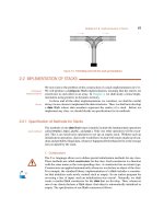
Figure 14.1

The Josephus problem: At each step, the darkest circle represents
the initial holder and the lightly shaded circle represents the player
who receives the hot potato (and is eliminated). Passes are made
clockwise.

was the sentence of death to the person next to the one who got the potato.
Josephus rigged the game to get the last lot and convinced the remaining
intended victim that the two of them should surrender. That is how we know
about this game; in effect, Josephus cheated.'
If M = 0, the players are eliminated in order, and the last player always
wins. For other values of M, things are not so obvious. Figure 14.1 shows
that if N = 5 and M = I, the players are eliminated in the order 2, 4, I , 5. In
this case, player 3 wins. The steps are as follows.

1. At the start, the potato is at player 1. After one pass it is at player 2.
2. Player 2 is eliminated. Player 3 picks up the potato, and after one
pass, it is at player 4.
3. Player 4 is eliminated. Player 5 picks up the potato and passes it to
player I.
4. Player I is eliminated. Player 3 picks up the potato and passes it to
player 5.
5. Player 5 is eliminated, so player 3 wins.
First, we write a program that simulates, pass for pass, a game for any
values of N and M. The running time of the simulation is O(MN), which is
acceptable if the number of passes is small. Each step takes O(M) time
because it performs M passes. We then show how to implement each step in
O(log N) time, regardless of the number of passes performed. The running
time of the simulation becomes O(N log N).

1. Thanks to David Teague for relaying this story. The version that we solve differs from the

historical description. In Exercise 14.12 you are asked to solve the historical version.


-

The Josephus Problem

14.1.I The Simple Solution
The passing stage in the Josephus problem suggests that we represent the
players in a linked list. We create a linked list in which the elements 1, 2,
. . . , N are inserted in order. We then set an iterator to the front element. Each
pass of the potato corresponds to a + + operation on the iterator. At the last
player (currently remaining) in the list we implement the pass by resetting
the iterator to the first element. This action mimics the circle. When we have
finished passing, we remove the element on which the iterator has landed.
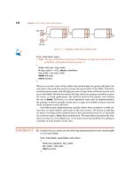
An implementation is shown in Figure 14.2 The linked list and iterator
are declared at lines 8 and 9, respectively. We construct the initial list by
using the loop at lines 14 and 15.
In Figure 14.2, the code at lines 20 to 33 plays one step of the algorithm
by passing the potato (lines 20 to 25) and then eliminating a player (lines
30-33). This procedure is repeated until the test at line 18 tells us that only
one player remains. At that point we return the player's number at line 36.
The running time of this routine is O ( M N ) because that is exactly the
number of passes that occur during the algorithm. For small M, this running
time is acceptable, although we should mention that the case M = 0 does not
yield a running time of O ( 0 ) ;obviously the running time is O(N).We do not
merely multiply by zero when trying to interpret a Big-Oh expression.

We can represent the
players by a linked

list and use the
iterator to
the passing.

14.1.2 A More Efficient Algorithm
A more efficient algorithm can be obtained if we use a data structure that supports accessing the kth smallest item (in logarithmic time). Doing so allows us
to implement each round of passing in a single operation. Figure 14.1 shows
why. Suppose that we have N players remaining and are currently at player P
from the front. Initially N is the total number of players and P is 1. After M
passes, a calculation tells us that we are at player ( ( P + M ) mod N) from the
front, except if that would give us player 0 , in which case, we go to player N.
The calculation is fairly tricky, but the concept is not.
Applying this calculation to Figure 14.1, we observe that M is 1, N is
initially 5, and P is initially 1. So the new value of P is 2. After the deletion,
N drops to 4, but we are still at position 2, as part (b) of the figure suggests.
The next value of P is 3, also shown in part (b), so the third element in the
list is deleted and N falls to 3. The next value of P is 4 mod 3, or 1, so we are
back at the first player in the remaining list, as shown in part (c). This player
is removed and N becomes 2. At this point, we add M to P, obtaining 2.
Because 2 mod 2 is 0 , we set P to player N, and thus the last player in the list
is the one that is removed. This action agrees with part (d). After the
removal, N is 1 and we are done.

If we implement each
round of passing in a
single logarithmic
operation, the
simulation will be
faster.

The calculation is
tricky because of the
circle.


1
2
3
4
5
6
7
8
9
10
11
12
13
14
15
16
17
18

#include <list>
using namespace std;
/ / Return the winner in the Josephus problem.
/ / STL list implementation.

int josephus( int people, int passes

list<int> thelist;
list<int>::iterator itr;
list<int>::iterator next;
int i;
/ / Construct the list.
for( i = 1; i <= people; i++
theList.push-back( i ) ;

20
21
22
23
24

!=

1; itr = next

)

{

++itr;
if( itr == theList.end( )
itr = theList.begin(

/ / Advance
)
);

/ / If past last player
/ / then go to first

1

25

next = itr;
++next;

/ / Maintain next node, for
/ / player who is after removed player

thelist .erase( itr

/ / Remove player

) ;

if( next == theList.end( )
next = theList.begin(

)

/ / Set next

) ;

1
return *itr;

/ / Return player's number

}

Figure 14.2

findKthcan be
supported by a
search tree.

)

/ / Play the game.
for( itr = theList.begin( ) ; people-i
for( i = 0; i < passes; i++ )

19

26
27
28
29
30
31
32
33
34
35
36

37

)

I

Linked list implementation of the Josephus problem.

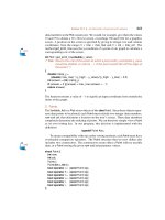
All we need then is a data structure that efficiently supports the f indKth
operation. The f indKth operation returns the kth (smallest) item, for any
parameter k.2 Unfortunately, no STL data structures support the f indKth
2. The parameter k for f indKth ranges from I to N, inclusive, where N is the number of
items in the data structure.


Event-Driven Simulation

operation. However, we can use one of the generic data structures that we
implement in Part IV. Recall from the discussion in Section 7.7 that the data
structures we implement in Chapter 19 follow a basic protocol that uses
insert,remove,and find.We can then add f indKth to the implementation.
There are several similar alternatives. All of them use the fact that, as discussed in Section 7.7, set could have supported the ranking operation in logarithmic time on average or logarithmic time in the worst case if we had used a
sophisticated binary search tree. Consequently, we can expect an O(N log N)
algorithm if we exercise care.
The simplest method is to insert the items sequentially into a worst-case
efficient binary search tree such as a red-black tree, an AA-tree, or a splay
tree (we discuss these trees in later chapters). We can then call findKth and
remove,as appropriate. It turns out that a splay tree is an excellent choice
for this application because the f indKth and insert operations are unusually efficient and remove is not terribly difficult to code. We use an alternative here, however, because the implementations of these data structures that
we provide in the later chapters leave implementing f indKth for you to do

as an exercise.
We use the BinarySearchTreeWi thRank class that supports the
f indKth operation and is completely implemented in Section 19.2. It is
based on the simple binary search tree and thus does not have logarithmic
worst-case performance but merely average-case performance. Conseauentlv. we cannot merelv insert the items seauentiallv:
, that would cause the
search tree to exhibit its worst-case performance.
There are several options. One is to insert a random permutation of 1, ...,
N into the search tree. The other is to build a perfectly balanced binary search
tree with a class method. Because a class method would have access to the
inner workings of the search tree, it could be done in linear time. This routine
is left for you to do as Exercise 19.21 when search trees are discussed.
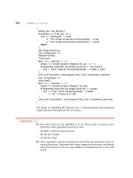
The method we use is to write a recursive routine that inserts items in a
balanced order. By inserting the middle item at the root and recursively
building the two subtrees in the same manner, we obtain a balanced tree. The
cost of our routine is an acceptable O(N log N).Although not as efficient as
the linear-time class routine, it does not adversely affect the asymptotic running time of the overall algorithm. The remove operations are then guaranteed to be logarithmic. This routine is called buildTree; it and the
j osephus method are then coded as shown in Figure 14.3.
2 ,

14.2 Event-Driven Simulation
Let us return to the bank simulation problem described in the introduction.
Here, we have a system in which customers arrive and wait in line until one

A balanced search
tree will work, but it is
not needed if we are
careful and construct
a simple binary
search tree that is not

unbalanced at the
start. A class method
can be used to
construct a perfectly
palanced tree in linear
time.

We construct the
Same tree by
recursive insertions
but use O(Nlog N)
time.


1
2
3
4
5
6
7
8
9
10
11
12
13
14
15
16

17
18
19
20
21
22
23
24
25
26
27
28
29
30
31
32
33
34
35
36
37

#include "BinarySearchTree.hN
/ / Recursively construct a perfectly balanced binary search
/ / tree by repeated insertions in O( N log N ) time.

void buildTree( BinarySearch~reeWithRank<int>& t,
int low, int high )
(

int center =

(

low + high

if ( low <= high

)

! 2;

)

I
t.insert( center ) ;
buildTree( t, low, center - 1 ) ;
buildTree ( t, center + 1 , high )

;

1
1
/ / Return the winner in the Josephus problem.
/ / Search tree implementation.

int josephus( int people, int passes

)

(

BinarySearchTree~ithRankiint>t;
buildTree( t, 1, people
int rank = 1;
while ( people > 1

);

)

{

if(

( rank = ( rank + passes
rank = people;

t.remove( t.findKth( rank
people-- ;

)

)

%

.get(

people

)

)

==

0 )

1;

1
return t.findKth( 1 ).get(

);

1

Figure 14.3

An O(N log N ) solution of the Josephus problem.

of k tellers is available. Customer arrival is governed by a probability distribution function, as is the service time (the amount of time to be served once
a teller becomes available). We are interested in statistics such as how long
on average a customer has to wait and what percentage of the time tellers are
actually servicing requests. (If there are too many tellers, some will not do
anything for long periods.)


Event-Driven ~ i r n u l a t i o n m

With certain probability distributions and values of k, we can compute
these answers exactly. However, as k gets larger the analysis becomes considerably more difficult and the use of a computer to simulate the operation
of the bank is extremely helpful. In this way, bank officers can determine
how many tellers are needed to ensure reasonably smooth service. Most simulations require a thorough knowledge of probability, statistics, and queueing theory.

14.2.1 Basic Ideas
A discrete event simulation consists of processing events. Here, the two
events are (1 ) a customer arriving and (2) a customer departing, thus freeing
up a teller.
We can use a probability function to generate an input stream consisting
of ordered pairs of arrival and service time for each customer, sorted by
arrival time.' We do not need to use the exact time of day. Rather, we can use
a quantum unit, referred to as a tick.
In a discrete time-driven simulation we might start a simulation clock
at zero ticks and advance the clock one tick at a time, checking to see
whether an event occurs. If so, we process the event(s) and compile statistics. When no customers are left in the input stream and all the tellers are
free, the simulation is over.
The problem with this simulation strategy is that its running time does
not depend on the number of customers or events (there are two events per
customer in this case). Rather, it depends on the number of ticks, which is
not really part of the input. To show why this condition is important, let us
change the clock units to microticks and multiply all the times in the input
by 1,000,000. The simulation would then take 1,000,000 times longer.
The key to avoiding this problem is to advance the clock to the next
event time at each stage, called an event-driven simulation, which is conceptually easy to do. At any point, the next event that can occur is either the
arrival of the next customer in the input stream or the departure of one of the
customers from a teller's station. All the times at which the events will happen are available, so we just need to find the event that happens soonest and
process that event (setting the current time to the time that the event occurs).
If the event is a departure, processing includes gathering statistics for the

departing customer and checking the line (queue) to determine whether
another customer is waiting. If so, we add that customer, process whatever

3. The probability function generates interarrival times (times between arrivals), thus guaranteeing that arrivals are generated chronologically.

The tick is the
quantum unit of time
in a simulation.

A discrete time-driven
simulation processes
each unit of time
consecutively. It is
inappropriate if the
interval between
successive events is
large.

An event-driven
simulation advances
the current time to the
next event.


The event set (i.e.,
events waiting to
happen) is organized
as a priority queue.

statistics are required, compute the time when the customer will leave, and

add that departure to the set of events waiting to happen.
If the event is an arrival, we check for an available teller. If there is none,
we place the arrival in the line (queue). Otherwise, we give the customer a
teller, compute the customer's departure time, and add the departure to the
set of events waiting to happen.
The waiting line for customers can be implemented as a queue. Because
we need to find the next soonest event, the set of events should be organized
in a priority queue. The next event is thus an arrival or departure (whichever
is sooner); both are easily available. An event-driven simulation is appropriate if the number of ticks between events is expected to be large.

14.2.2 Example: A Modem Bank Simulation
The main algorithmic item in a simulation is the organization of the events
in a priority queue. To focus on this requirement, we write a simple simulation. The system we simulate is a nzodeni bank at a university computing
center.
A modem bank consists of a large collection of modems. For example,
Florida International University (FIU) has 288 modems a\iailable for students. A modem is accessed by dialing one telephone number. If any
of the 288 modems are available, the user is connected to one of them. If all
the modems are in use, the phone will give a busy signal. Our simulation
models the service provided by the modem bank. The variables are
the number of modems in the bank,
the probability distribution that governs dial-in attempts,
the probability distribution that governs connect time, and
the length of time the simulation is to be run.
The modem bank
the waiting
line from the
simulation.Thus
there is only one data
structure.

We list each event as
it
gathering
statistics is a simple
extension.

The modem bank simulation is a simplified version of the bank teller
simulation because there is no waiting line. Each dial-in is an arrival, and the
total time spent once a connection has been established is the service time.
By removing the waiting line, we remove the need to maintain a queue. Thus
we have only one data structure, the priority queue. In Exercise 14.18 you
are asked to incorporate a queue; as many as L calls will be queued if all the
modems are busy.
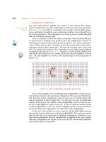
To simplify matters, we do not compute statistics. Instead, we list each
event as it is processed. We also assume that attempts to connect occur at constant intervals; in an accurate simulation? we would model this interarrival
time by a random process. Figure 14.4 shows the output of a simulation.


--

-

Event-Driven Slmulatlon

1 User 0 dials in at time 0 and connects for 1 minutes
2 User 0 hangs up at time 1
3 user 1 dials in at time 1 and connects for 5 minutes
4 user 2 dials in at time 2 and connects for 4 minutes
5 User 3 dials in at time 3 and connects for 11 minutes
6 user 4 dials in at time 4 but gets busy signal

7 user 5 dials in at time 5 but gets busy signal
8 user 6 dials in at time 6 but gets busy signal
9 User 1 hangs up at time 6
10 User 2 hangs up at time 6
11 User 7 dlals in at time 7 and connects for 8 minutes
12 User 8 dials in at time 8 and connects for 6 minutes
13 User 9 dials in at time 9 but gets busy signal
14 User 10 dials in at time 10 but gets busy signal
15 User 11 dials in at time 11 but gets busy signal
16 User 12 dials in at time 12 but gets busy signal
17 User 13 dials in at time 13 but gets busy signal
18 User 3 hangs up at time 14
19 User 14 dials in at time 14 and connects for 6 minutes
20 User 8 hangs up at time 14
21 User 15 dials in at time 15 and connects for 3 minutes
22 User 7 hangs up at time 15
23 User 16 dials in at time 16 and connects for 5 minutes
24 user 17 dials in at time 17 but gets busy signal
25 User 15 hangs up at time 18
26 User 18 dials in at time 18 and connects for 7 minutes
Figure 14.4

Sample output for the modem bank simulation involving three
modems: A dial-in is attempted every minute; the average connect
time is 5 minutes; and the simulation is run for 18 minutes.

The simulation class requires another class to represent events. The
Event class is shown in Figure 14.5. The data members consist of the customer number, the time that the event will occur. and an indication of what
type of event (DIAL-IN or HANG-UP) it is. If this simulation were more
complex, with several types of events, we would make Event an abstract

base class and derive subclasses from it. We do not do that here because that
would complicate things and obscure the basic workings of the simulation
algorithm. The Event class contains a constructor and a comparison function used by the priority queue. The Event class grants friendship status to
the modem simulation class so that vent's internal members can be
accessed by ModemSim methods.
The modem simulation class, ModemSim, is shown in Figure 14.6. It
consists of a lot of data members, a constructor, and two member functions.
The data members include a random number object r shown at line 25. At

The Event class
represents events. In
a complex simulation,
it would derive all
possible types of
events as subclasses.
Using inheritance for
the Event class
would complicate the
code.


1
2
3
4
5
6
7
8
9

10
11
12
13
14
15
16
17
18
19
20
21
22
23
24

#include <limits.h>
#include <time.h>
#include <stdlib.h>
#include "Random.hU
#include <iostream>
#include <vector>
#include <queue>
#include <functional>
using namespace std;
class Event
{

25
26

27 } ;

enum { DIAL-IN = 1, HANG-UP = 2 1 ;
public:
Event( int name = 0 , int tm = 0 , int type = DIAL-IN 1
: time( tm ) , who( name ) , what( type ) i 1
boo1 operator> ( const Event & rhs
{ return time > rhs.time; 1

const

friend class ModemSim;
private:
int who;
int time ;
int what;

Figure 14.5

The nextcall
function adds a dialin request to the
event set.

)

/ / the number of the user

/ I when the event will occur
/ / DIAL-IN or HANG-UP

The Event class used for modem simulation.

line 26 the eventset is maintained as a priority queue of Event
objects ( P Q is a typedef, given at line 10, that hides a complicated
priority-queue template instantiation). The remaining data members are
freeModems,which is initially the number of modems in the simulation but
changes as users connect and hang up, and avgCallLen and freqofcalls,
which are parameters of the simulation. Recall that a dial-in attempt will be
made every f reqofcalls ticks. The constructor, declared at line 15, and
implemented in Figure 14.7 initializes these members and places the first
arrival in the eventset priority queue.
The simulation class consists of only two member functions. First,
nextcall,shown in Figure 14.8 adds a dial-in request to the event set. It
maintains two static variables: the number of the next user who will attempt
to dial in and when that event will occur. Again, we have made the simplifying assumption that calls are made at regular intervals. In practice, we would
use a random number generator to model the arrival stream.


Event-Driven Simulation

1
2
3
4
5
6
7

/ / ModemSim class interface: run a simulation.
//

/ / CONSTRUCTION: with three parameters: the number of
//
modems, the average connect time, and the
//
inter-arrival time.
//
/ / ******************PUBLIC
OPEmTIONS*********************

8 / / void runSim( )

-->

Run a simulation

9
10 typedef priority~queue> PQ;
11
12 class ModemSim
13 {
14
public:
15
ModemSim( int modems, double avgLen, int callIntrv1 ) ;
16
/ / Add a call to eventset at the current time,
17
18
/ / and schedule one for delta in the future.

19
void nextcall( int delta ) ;
20
21
/ / Run the simulation.
22
void runSim( int stoppingTime = INT-MAX ) ;
23
private:
24
25
Random r;
/ / A random source
26
PQ eventset;
/ / Pending events
27
/ / Basic parameters of the simulation.
28
29
int freeModems;
/ / Number of modems unused
30
const double avgCallLen;
/ / Length of a call
31
const int freq0fCalls;
/ / Interval between calls
32 } ;
Figure 14.6

The ModemSim class interface.

1 / / Constructor for ModemSim.
2 ModemSim::ModemSim( int modems, double avglen, int callIntrvl
3
: freeModems( modems ) , avgCallLen( avgLen ) ,
4
freqOfCalls( callIntrvl ) , r( (int) time( 0 ) )
5 {
6
nextcall( freqofcalls ) ;
/ / Schedule first call
7 }
Figure 14.7

The ModemSim constructor.

)


Simulation
1 / / Place a new DIAL-IN event into the event queue.
2 / / Then advance the time when next DIAL-IN event will occur.
3 / / In practice, we would use a random number to set the time.
4 void ModemSim::nextCall( int delta 1
5 {
6
static int nextCallTime = 0;
7

static int userNum = 0;
8
9
eventSet.push( Event( userNum++, nextCallTime ) ) ;
10
nextCallTime += delta;
11 }

Figure 14.8

The runSim function
runs the simulation.

A hang-up increases
freeModems.A dialin checks on whether
a modem is available
and if so decreases

f reeModems.

The nextcall function places a new DIAL-IN event in the event
queue and advances the time when the next DIAL-IN event will occur.

The other member function is runsim,which is called to run the entire
simulation. The runsim function does most of the work and is shown in
Figure 14.9. It is called with a single parameter that indicates when the simulation should end. As long as the event set is not empty, we process events.
Note that it should never be empty because at the time we arrive at line 10
there is exactly one dial-in request in the priority queue and one hang-up
request for every currently connected modem. Whenever we remove an
event at line 10 and it is confirmed to be a dial-in, we generate a replacement

dial-in event at line 37. A hang-up event is also generated at line 32 if the
dial-in succeeds. Thus the only way to finish the routine is if nextcall is
set up not to generate an event eventually or (more likely) by executing the
break statement at line 12.
Let us summarize how the various events are processed. If the event is a
hang-up, we increment f reeModems at line 16 and print a message at line 17.
If the event is a dial-in, we generate a partial line of output that records the
attempt, and then, if any modems are available, we connect the user. To do so,
we decrement freeModems at line 26,generate a connection time (using a
Poisson distribution rather than a uniform distribution) at line 27, print the rest
of the output at line 28, and add a hang-up to the event set (lines 30-32). Otherwise, no modems are available, and we give the busy signal message. Either
way, an additional dial-in event is generated. Figure 14.10 shows the state of
the priority queue after each deleteMin for the early stages of the sample
output shown in Figure 14.4. The time at which each event occurs is shown in
boldface, and the number of free modems (if any) are shown to the right of the
priority queue. (Note that the call length is not actually stored in an Event
object; we include it, when appropriate to make the figure more self-contained.
A '?' for the call length signifies a dial-in event that eventually will result in a
busy signal; however, that outcome is not known at the time the event is added
to the priority queue.) The sequence of priority queue steps is as follows.


Event-Driven Simulation
1
2
3
4
5
6
7

8
9
10
11
12
13
14
15
16
17
18
19
20
21
22
23
24
25
26
27
28
29
30
31
32
33
34
35
36
37

38
39
40

/ / Run the simulation until stopping time occurs.
/ / Print output as in Figure 14.4.

void ModemSim::runSim( int stoppingTime
I
static Event e;
int howlong;
while( !eventSet.empty( )

)

)

{

e = eventSet.top( ) ; eventSet.pop(
if( e.time > stoppingTime )
break;
if( e.what == Event::HANG-UP

)

);

l i HANG-UP

{

freeModems++;
cout << "User
<< e.who < < " hangs up at time "
< < e.time << endl;
'I

}

else

/ / DIAL-IN

{

cout << "User " << e.who << " dials in at time
<< e.time <<
";
if( freeModems > 0 )
!
freeModems--;
howLong = r.poisson( avgCallLen ) ;
cout << "and connects for "
<< howLong <<
minutes" < < endl;
e.tirne + = howlong;
e.what = Event::HANG-UP;
eventset .push( e ) ;
1

else
cout << "but gets busy signal" < < endl;
I'

"

nextcall( freqOfCalls 1 ;
1

1
1

Figure 14.9

The basic simulation routine.

1. The first DIAL-IN request is inserted.
2. After DIAL-IN is removed, the request is connected, thereby resulting in a HANG-UP and a replacement DIAL-IN request.
3. A HANG-UP request is processed.
4. A DIAL-IN request is processed resulting in a connect. Thus both a
HANG-UP event and a DIAL-IN event are added (three times).

"


User 0, Len 1

User 1, Len 5

User 1, Len 5

User 2. Len 4

User I. Len 5

User 2, Len 4

User 3. Len 1 L

User I , Len 5

User 2, Len 4

User 3, Len 11

User 1, Len 5

User 2. Len 4

1 4 u s e r 3,

User 2, Len 4

User I , Len 5

User 2, Len 4

User 4, Len ?

II

v
lm)

(1
6
User 1, Len 5

en

1

en I I

User 6, Len ?

User 3. Len 1 1

User 7, Len 8

1 4 u s e r 3,

User 2, Len 4

User 3, Len 1 1

User 7, Len 8

Figure 14.10 The priority queue for modem bank simulation after each step.

--

Event-Driven Simulation

5. A DIAL-IN request fails; a replacement DIAL-IN is generated
(three times).
6. A HANG-UP request is processed (twice).
7. A DIAL-IN request succeeds, and HANG-UP and DIAL-IN are
added.
Again, if Event were an abstract base class, we would expect a procedure doEvent to be defined through the Event hierarchy; then we would
not need long chains of if /else statements. However to access the priority
queue, which is in the simulation class, we would need Event to store a
pointer to the simulation ModemSim class as a data member. We would insert
it at construction time.
A minimal main routine is shown for completeness in Figure
- 14.1 1 .
However, using a Poisson distribution to model connect time is not appropriate. A better choice would be to use a negative exponential distribution (but
the reasons for doing so are beyond the scope of this text). Additionally,
assuming a fixed time between dial-in attempts is also inaccurate. Again, a
negative exponential distribution would be a better model. If we change the
simulation to use these distributions, the clock would be represented as a
double. In Exercise 14.14 you are asked to implement these changes.

Thesimulation usesa
poor model. Negative
exponential
distributions would
more accurately
model the time

between dial-in
attempts and total
connect time.

1 / / Simple main to test ModemSim class.
2 int main( )
3 {
4
int numModems;
5
int totalTime;
6
double avgConnectTime;
7
int dialInFrequency;
8
9
cout << "Enter: number of modems, length of simulation, "
10
< < " average connect time, how often calls occur: " ;
11
12
cin >> numModems >> totalTime >>
13
avgConnectTime >> dialInFrequency;
14
15
ModemSim s( numModems, avgConnectTime, dialInFrequency ) ;
16
s.runSim( totalTime ) ;

17
return 0;
18
19 1

Figure 14.11 A simple main to test the simulation.


Summary
Simulation is an important area of computer science and involves many
more complexities than we could discuss here. A simulation is only as good
as the model of randomness, so a solid background in probability, statistics,
and queueing theory is required in order for the modeler to know what types
of probability distributions are reasonable to assume. Simulation is an
important application area for object-oriented techniques.

Objects of the Game
discrete time-driven simulation A simulation in which each unit of
time is processed consecutively. It is inappropriate if the interval
between successive events is large. (p. 477)
event-driven simulation A simulation in which the current time is
advanced to the next event. (p. 477)
Josephus problem A game in which a hot potato is repeatedly passed;
when passing terminates, the player holding the potato is eliminated; the game then continues, and the last remaining player wins.
(P. 47 1)
simulation An important use of computers, in which the computer is
used to emulate the operation of a real system and gather statistics.
(P. 47 1)
tick The quantum unit of time in a simulation. (p. 477)

@
/

Common Errors
1. The most common error in simulation is using a poor model. A simulation is only as good as the accuracy of its random input.

On the Internet
-

Both examples in this chapter are available online.

Josephus.cpp Contains both implementations of j osephus and a
main to test them.
Modems.cpp Contains the code for the modem bank simulation.

Q

Exercises

-

In Short
14.1. If M = 0, who wins the Josephus game?


Show the operation of the Josephus algorithm in Figure 14.3 for the
case of seven people with three passes. Include the computation of
r a n k and a picture that contains the remaining elements after each
iteration.
Are there any values of M for which player 1 wins a 30-person Josephus game?

Show the state of the priority queue after each of the first 10 lines of
the simulation depicted in Figure 14.4.

In Theory
Let N = 2"or
any integer k . Prove that if M is 1, then player 1
always wins the Josephus game.
Let J(N) be the winner of an N-player Josephus game with M = 1.
Show that
a. if N is even. then J(h? = 2 J ( N l 2 ) - I.
b. if N is odd and J ( r ~ 1 2 1 #) 1. then J(N) = 2J(rNl 21) - 3.
c. if N is odd and J ( r N 121) = I , then J ( N ) = N.
Use the results in Exercise 14.6 to write an algorithm that returns the
winner of an N-player Josephus game with M = I . What is the running time of your algorithm'?
Give a general formula for the winner of an N-player Josephus game
with M = 2.
Using the algorithm for N = 20, determine the order of insertion into
the~inar~search~ree~ith~ank.

In Practice
Suppose that the Josephus algorithm shown in Figure 14.2 is implemented with a v e c t o r instead of a 1i s t .
a. If the change worked, what would be the running time?
b. The change has a subtle error. What is the problem and how can
it be fixed?
In the Josephus algorithm shown in Figure 14.2, why can't we
replace lines 27 and 28 with the single assignment n e x t = i t r +l?
Write a program that solves the historical version of the Josephus
problem. Give both the linked list and search tree algorithms.
Implement the Josephus algorithm with a queue. Each pass of the
potato is a dequeue. followed by an enqueue.

14.14. Rework the simulation so that the clock is represented as a double.
the time between dial-in attempts is modeled with a negative exponential distribution, and the connect time is modeled with a negative
exponential distribution.
14.15. Rework the modem bank simulation so that Event is an abstract
base class and DialInEvent and HangUpEvent are derived
classes. The Event class should store a pointer to a ModemSim
object as an additional data member, which is initialized on construction. It should also provide an abstract method named doEvent
that is implemented in the derived classes and that can be called
from runsim to process the event.
Programming Projects

14.16. Implement the Josephus algorithm with splay trees (see Chapter 22)
and sequential insertion. (The splay tree class is available online, but
it will need a findKth method.) Compare the performance with
that in the text and with an algorithm that uses a linear-time, balanced tree-building algorithm.
14.17. Rewrite the Josephus algorithm shown in Figure 14.3 to use a
median heap (see Exercise 7.19). Use a simple implementation of
the median heap; the elements are maintained in sorted order. Compare the running time of this algorithm with the time obtained by
using the binary search tree.
14.18. Suppose that FIU has installed a system that queues phone calls
when all modems are busy. Rewrite the simulation routine to allow
for queues of various sizes. Make an allowance for an infinite queue.
14.19. Rewrite the modem bank simulation to gather statistics rather than
output each event. Then compare the speed of the simulation,
assuming several hundred modems and a very long simulation, with
some other possible priority queues (some of which are available
online)-namely, the following.
a. An asymptotically inefficient priority queue representation

described in Exercise 7.14.
b. An asymptotically inefficient priority queue representation
described in Exercise 7.15.
c. Splay trees (see Chapter 22).
d. Skew heaps (see Chapter 23).
e. Pairing heaps (see Chapter 23).


Chapter 15

I Graphs and Paths
In this chapter we examine the graph and show how to solve a particular
kind of problem-namely, calculation of shortest paths. The computation of
shortest paths is a fundamental application in computer science because
many interesting situations can be modeled by a graph. Finding the fastest
routes for a mass transportation system, and routing electronic mail through
a network of computers are but a few examples. We examine variations of
the shortest path problems that depend on an interpretation of shortest and
the graph's propertjes. Shortest-path problems are interesting because,
although the algorithms are fairly simple, they are slow for large graphs
unless careful attention is paid to the choice of data structures.
In this chapter, we show:
formal definitjons of a graph and its components.
the data structures used to represent a graph, and
algorithms for solving several variations of the shortest-path problem,
with complete C++ implementations.

Definitions
A graph consists of a set of vertices and a set of edges that connect the vertices. That is, G =
E),where V is the set of v e k c e s and E is the set of

edges. Each edge is a pair (v, w),where v, w E \! Vertices are sometimes
called nodes, and edges are sometimes called arcs. If the edge pair is
ordered, the graph is called a directed graph. Directed graphs aresometimes called digraphs. In a digraph, vertex w is adjacent to vertex v if and
only if (v, w ) E E.Sometimes an edge has a third component, called the edge
cost (or weight) that measures the cost of traversing the edge. In this chapter, all graphs are directed.

(v

A graph consists of a
Set Of vertices and a
set of edges that
connect the vertices,
~ftheedge pair is
ordered7thegraph is
a directed graph.
Vertex w i s adjacent
to vertex vif there is
an edge from v to w.


Graphs and Paths

Figure 15.1

A directed graph

The graph shown in Figure 15.1 has seven vertices,

v

= { v o , v , , v,, v,, v,,

v,, V6 I-,

and 12 edges,

A path is a sequence
of vertices connected
by edges.

The unweighted path
length measures the
number of edges on a
path.
The weighted path
length is the sum of
the edge costs on a
path.

A cycle in a directed
graph is a path that
begins and ends at
the same vertex and
contains at least one
edge.

The following vertices are adjacent to V3: VZ.V4, V,, and V6. Note that V, and
V, are not adjacent to V3. For this graph, / VI = 7 and IEl = 12; here, IS1
represents the size of set S .
A path in a graph is a sequence of vertices connected by edges. In other

words, w , ,w2,. . ., wh,the sequence of vertices is such that ( w , , w i E E
for I 5 i < N. The path length is the number of edges on the path-namely,
N - I-also called the unweighted path length. The weighted path length
is the sum of the costs of the edges on the path. For example, Vo, V,, V5 is a
path from vertex Vo to V 5 .The path length is two edges-the shortest path
between Vo and V,, and the weighted path length is 9. However, if cost is
important, the weighted shortest path between these vertices has cost 6 and
is Vo, V,, V,, V, . A path may exist from a vertex to itself. If this path contains no edges, the path length is 0, which is a convenient way to define an
otherwise special case. A simple path is a path in which all vertices are distinct, except that the first and last vertices can be the same.
A cycle in a directed graph is a path that begins and ends at the same
vertex and contains at least one edge. That is, it has a length of at least 1 such
that w , = w,,,;this cycle is simple if the path is simple. A directed acyclic
graph (DAG) is a type of directed graph having no cycles.
+


An example of a real-life situation that can be modeled by a graph is the
airport system. Each airport is a vertex. If there is a nonstop flight between
two airports, two vertices are connected by an edge. The edge could have a
weight, representing time, distance, or the cost of the flight. In an undirected
graph, an edge ( v , w) would imply an edge (w, v). However, the costs of the
edges might be different because flying in different directions might take
longer (depending on prevailing winds) or cost more (depending on local
taxes). Thus we use a directed graph with both edges listed, possibly with
different weights. Naturally, we want to determine quickly the best flight
between any two airports; best could mean the path with the fewest edges or
one, or all, of the weight measures (distance, cost, and so on).
A second example of a real-life situation that can be modeled by a graph
is the routing of electronic mail through computer networks. Vertices represent computers, the edges represent links between pairs of computers, and the
edge costs represent communication costs (phone bill per megabyte), delay

costs (seconds per megabyte), or combinations of these and other factors.
For most graphs, there is likely at most one edge from any vertex v
to any other vertex w (allowing one edge in each direction between v and
w).Consequently, 1E 6 ( ~ 1 ' .When most edges are present, we have
1El = O ( / V /'). Such a graph is considered to be a dense graph-that is, it
has a large number of edges, generally quadratic.
In most applications, however, a sparse graph is the norm. For instance,
in the airport model, we do not expect direct flights between every pair of
airports. Instead, a few airports are very well connected and most others
have relatively few flights. In a complex mass transportation system involving buses and trains, for any one station we have only a few other stations
that are directly reachable and thus represented by an edge. Moreover, in a
computer network most computers are attached to a few other local computers. So, in most cases, the graph is relatively sparse, where IEl = @(IV ) or
perhaps slightly more (there is no standard definition of sparse). The algorithms that we develop, then, must be efficient for sparse graphs.

15.1 .1

A directedacyclic
graph has no cycles.
Such graphs are an
important class of
graphs.

A graph is dense if
Of edges
the
is large (generally
quadratic,.Typical
graphs are not dense.
Instead, they are
sparse.

Representation

The first thing to consider is how to represent a graph internally. Assume that
the vertices are sequentially numbered starting from 0, as the graph shown in
Figure 15.1 suggests. One simple way to represent a graph is to use a twodimensional array called an adjacency matrix. For each edge (v, w), we set
a [v][ w ] equal to the edge cost; nonexistent edges can be initialized with a
logical INFINITY.The initialization of the graph seems to require that the
entire adjacency matrix be initialized to INFINITY.Then, as an edge is
encountered, an appropriate entry is set. In this scenario, the initialization

An adjacency matrix
represents a graph
and uses quadratic
space.


Graphs and Paths

Figure 15.2

An adjacency list
represents a graph,
using linear space.

Adjacency lists can
be constructed in
linear time from a list
of edges.

Adjacency list representation of the graph shown in Figure 15.1 ; the
nodes in list i represent vertices adjacent to iand the cost of the
connecting edge.

takes O(IVI2) time. Although the quadratic initialization cost can be
avoided (see Exercise 15.6), the space cost is still 0(1VI2), which is fine for
dense graphs but completely unacceptable for sparse graphs.
For sparse graphs, a better solution is an adjacency list, which represents
a graph by using linear space. For each vertex, we keep a list of all adjacent
vertices. An adjacency list representation of the graph in Figure 15.1 using a
linked list is shown in Figure 15.2. Because each edge appears in a list node,
the number of list nodes equals the number of edges. Consequently, O(IE1)
space is used to store the list nodes. We have IVI lists, so O(IVJ) additional
space is also required. If we assume that every vertex is in some edge, the
number of edges is at least rlV1/21. Hence we may disregard any O(IV1)
terms when an O(IE1) term is present. Consequently, we say that the space
requirement is O(IEI), or linear in the size of the graph.
The adjacency list can be constructed in linear time from a list of edges.
We begin by making all the lists empty. When we encounter an edge
(v, W, c,,,,), we add an entry consisting of w and the cost c , ,to v's adjacency list. The insertion can be anywhere; inserting it at the front can be done
in constant time. Each edge can be inserted in constant time, so the entire adjacency list structure can be constructed in linear time. Note that when inserting
an edge, we do not check whether it is already present. That cannot be done in
constant time (using a simple linked list), and doing the check would destroy
the linear-time bound for construction. In most cases, ignoring this check is


unimportant. If there are two or more edges of different cost connecting a pair
of vertices, any shortest-path algorithm will choose the lower cost edge
without resorting to any special processing. Note also that v e c t o r s can be
used instead of linked lists, with the constant-time push-back operation

replacing insertions at the front.
In most real-life applications the vertices have names, which are
unknown at compile time, instead of numbers. Consequently, we must provide a way to transform names to numbers. The easiest way to do so is to
provide a map by which we map a vertex name to an internal number ranging from 0 to IV - 1 (the number of vertices is determined as the program
runs). The internal numbers are assigned as the graph is read. The first
number assigned is 0. As each edge is input, we check whether each of the
two vertices has been assigned a number, by looking in the map. If it has
been assigned an internal number, we use it. Otherwise, we assign to the
vertex the next available number and insert the vertex name and number in
the map. With this transformation, all the graph algorithms use only the
internal numbers. Eventually, we have to output the real vertex names, not
the internal numbers, so for each internal number we must also record the
corresponding vertex name. One way to do so is to keep a string for each
vertex. We use this technique to implement a G r a p h class. The class and
the shortest path algorithms require several data structures-namely, list, a
queue? a map, and a priority queue. The # i n c l u d e directives for system
headers are shown in Figure 15.3. The queue (implemented with a linked
list) and priority queue are used in various shortest-path calculations. The
adjacency list is represented with v e c t o r s . A map is also used to represent
the graph.
When we write an actual C++ implementation, we do not need internal
vertex numbers. Instead, each vertex is stored in a V e r t e x object, and
instead of using a number, we can use the address of the v e r t e x object as
its (uniquely identifying) number. As a result, the code makes frequent use

Figure 15.3

The

# i n c l u d e directives for the Graph class.

A map can be used to
map vertex names to
internal numbers.


of vertex* variables. However, when describing the algorithms, assuming
that vertices are numbered is often convenient, and we occasionally do so.
Before we show the Graph class interface, let us examine Figures 15.4
and 15.5, which show how our graph is to be represented. Figure 15.4 shows
the representation in which we use internal numbers. Figure 15.5 replaces
the internal numbers with vertex* variables, as we do in our code.
Although this simplifies the code. it greatly complicates the picture. Because
the two figures represent identical inputs, Figure 15.4 can be used to follow
the complications in Figure 15.5.
t . can expect the user to provide a
As indicated in the part labeled I n p ~ ~we
list of edges, one per line. At the start of the algorithm, we do not know the
names of any of the vertices. how many vertices there are, or how many edges
there are. We use two basic data structures to represent the graph. As we mentioned in the preceding paragraph, for each vertex we maintain a vertex
object that stores some information. We describe the details of vertex (in
particular, how different vertex objects interact with each other) last.
As mentioned earlier. the first major data structure is a map that allows
us to find, for any vertex name, a pointer to the vertex object that represents it. This map is shown in Figure 15.5 as vertexMap (Figure 15.4 maps
the name to an i n t in the component labeled Dictionan).

dist Drev name

adi

2
C

A 19
Input

3
4

Visual repvesentarioi? of graph
Figure 15.4

Dictiorzap

An abstract scenario of the data structures used in a shortest-path
calculation, with an input graph taken from a file. The shortest
weighted path from A to C is A to B to E to D to C (cost is 76).


&

19

10

43

Visual representation of graph
Input
r

-

-

i

Legend: Dark-bordered boxes are vertex objects. The unshaded portion
in each box contains the name and adjacency list and does not change
when shortest-path computation is performed. Each adjacency list entry
contains an Edge that stores a pointer to another vertex object and the
edge cost. Shaded portion is d i s t and prev, Jilled in after shortest path
computation runs.
Dark pointers emanate from ver t emap Light pointers are adjacency
list entries. Dashed-pointers are the prev data member that results from a
shortest path computation.
Figure 15.5

Data structures used in a shortest-path calculation, with an input
graph taken from a file; the shortest weighted path from A to C is:
A to B to E to D to C (cost is 76).