Ebook Data structures and algorithms in C++: Part 2

✐

✐

“main” — 2011/1/13 — 9:10 — page 321 — #343
✐

✐

Chapter

8

Heaps and Priority Queues

Contents
8.1

8.2

8.3

The Priority Queue Abstract Data Type . . . . . . . .
8.1.1 Keys, Priorities, and Total Order Relations . . . . . .
8.1.2 Comparators . . . . . . . . . . . . . . . . . . . . . .
8.1.3 The Priority Queue ADT . . . . . . . . . . . . . . .
8.1.4 A C++ Priority Queue Interface . . . . . . . . . . . .
8.1.5 Sorting with a Priority Queue . . . . . . . . . . . . .
8.1.6 The STL priority queue Class . . . . . . . . . . . . .
Implementing a Priority Queue with a List . . . . . .
8.2.1 A C++ Priority Queue Implementation using a List .

8.2.2 Selection-Sort and Insertion-Sort . . . . . . . . . . .
Heaps . . . . . . . . . . . . . . . . . . . . . . . . . . .
8.3.1 The Heap Data Structure . . . . . . . . . . . . . . .
8.3.2 Complete Binary Trees and Their Representation . .
8.3.3 Implementing a Priority Queue with a Heap . . . . .
8.3.4 C++ Implementation . . . . . . . . . . . . . . . . .
8.3.5 Heap-Sort . . . . . . . . . . . . . . . . . . . . . . .
8.3.6 Bottom-Up Heap Construction
. . . . . . . . . .
Adaptable Priority Queues . . . . . . . . . . . . . . .
8.4.1 A List-Based Implementation . . . . . . . . . . . . .
8.4.2 Location-Aware Entries . . . . . . . . . . . . . . . .
Exercises . . . . . . . . . . . . . . . . . . . . . . . . .

⋆

8.4

8.5

322
322
324
327
328
329
330
331
333
335

337
337
340
344
349
351
353
357
358
360
361

✐

✐
✐

✐


✐

✐

“main” — 2011/1/13 — 9:10 — page 322 — #344
✐

✐

322

8.1

Chapter 8. Heaps and Priority Queues

The Priority Queue Abstract Data Type
A priority queue is an abstract data type for storing a collection of prioritized elements that supports arbitrary element insertion but supports removal of elements in
order of priority, that is, the element with first priority can be removed at any time.
This ADT is fundamentally different from the position-based data structures such
as stacks, queues, deques, lists, and even trees, we discussed in previous chapters.
These other data structures store elements at specific positions, which are often
positions in a linear arrangement of the elements determined by the insertion and
deletion operations performed. The priority queue ADT stores elements according
to their priorities, and has no external notion of “position.”

8.1.1 Keys, Priorities, and Total Order Relations
Applications commonly require comparing and ranking objects according to parameters or properties, called “keys,” that are assigned to each object in a collection. Formally, we define a key to be an object that is assigned to an element as a
specific attribute for that element and that can be used to identify, rank, or weigh
that element. Note that the key is assigned to an element, typically by a user or application; hence, a key might represent a property that an element did not originally
possess.
The key an application assigns to an element is not necessarily unique, however,
and an application may even change an element’s key if it needs to. For example,
we can compare companies by earnings or by number of employees; hence, either
of these parameters can be used as a key for a company, depending on the information we wish to extract. Likewise, we can compare restaurants by a critic’s food
quality rating or by average entr´ee price. To achieve the most generality then, we
allow a key to be of any type that is appropriate for a particular application.
As in the examples above, the key used for comparisons is often more than
a single numerical value, such as price, length, weight, or speed. That is, a key
can sometimes be a more complex property that cannot be quantified with a single
number. For example, the priority of standby passengers is usually determined by

taking into account a host of different factors, including frequent-flyer status, the
fare paid, and check-in time. In some applications, the key for an object is data
extracted from the object itself (for example, it might be a member variable storing
the list price of a book, or the weight of a car). In other applications, the key is not
part of the object but is externally generated by the application (for example, the
quality rating given to a stock by a financial analyst, or the priority assigned to a
standby passenger by a gate agent).

✐

✐
✐

✐


✐

✐

“main” — 2011/1/13 — 9:10 — page 323 — #345
✐

✐

8.1. The Priority Queue Abstract Data Type

323

Comparing Keys with Total Orders

A priority queue needs a comparison rule that never contradicts itself. In order for
a comparison rule, which we denote by ≤, to be robust in this way, it must define
a total order relation, which is to say that the comparison rule is defined for every
pair of keys and it must satisfy the following properties:
• Reflexive property : k ≤ k
• Antisymmetric property: if k1 ≤ k2 and k2 ≤ k1 , then k1 = k2
• Transitive property: if k1 ≤ k2 and k2 ≤ k3 , then k1 ≤ k3

Any comparison rule, ≤, that satisfies these three properties never leads to a
comparison contradiction. In fact, such a rule defines a linear ordering relationship
among a set of keys. If a finite collection of keys has a total order defined for it, then
the notion of the smallest key, kmin , is well defined as the key, such that kmin ≤ k,
for any other key k in our collection.
A priority queue is a container of elements, each associated with a key. The
name “priority queue” comes from the fact that keys determine the “priority” used
to pick elements to be removed. The fundamental functions of a priority queue P
are as follows:
insert(e): Insert the element e (with an implicit associated key value)
into P.
min(): Return an element of P with the smallest associated key
value, that is, an element whose key is less than or equal
to that of every other element in P.
removeMin(): Remove from P the element min().
Note that more than one element can have the same key, which is why we were
careful to define removeMin to remove not just any minimum element, but the
same element returned by min. Some people refer to the removeMin function as
extractMin.
There are many applications where operations insert and removeMin play an
important role. We consider such an application in the example that follows.
Example 8.1: Suppose a certain flight is fully booked an hour prior to departure.

Because of the possibility of cancellations, the airline maintains a priority queue of
standby passengers hoping to get a seat. The priority of each passenger is determined by the fare paid, the frequent-flyer status, and the time when the passenger is
inserted into the priority queue. When a passenger requests to fly standby, the associated passenger object is inserted into the priority queue with an insert operation.
Shortly before the flight departure, if seats become available (for example, due to
last-minute cancellations), the airline repeatedly removes a standby passenger with
first priority from the priority queue, using a combination of min and removeMin
operations, and lets this person board.

✐

✐
✐

✐


✐

✐

“main” — 2011/1/13 — 9:10 — page 324 — #346
✐

✐

Chapter 8. Heaps and Priority Queues

324

8.1.2 Comparators

An important issue in the priority queue ADT that we have so far left undefined
is how to specify the total order relation for comparing the keys associated with
each element. There are a number of ways of doing this, each having its particular
advantages and disadvantages.
The most direct solution is to implement a different priority queue based on
the element type and the manner of comparing elements. While this approach is
arguably simple, it is certainly not very general, since it would require that we
make many copies of essentially the same code. Maintaining multiple copies of the
nearly equivalent code is messy and error prone.
A better approach would be to design the priority queue as a templated class,
where the element type is specified by an abstract template argument, say E. We
assume that each concrete class that could serve as an element of our priority queue
provides a means for comparing two objects of type E. This could be done in
many ways. Perhaps we require that each object of type E provides a function
called comp that compares two objects of type E and determines which is larger.
Perhaps we require that the programmer defines a function that overloads the C++
comparison operator “<” for two objects of type E. (Recall Section 1.4.2 for a
discussion of operator overloading). In C++ jargon this is called a function object.
Let us consider a more concrete example. Suppose that class Point2D defines a
two-dimensional point. It has two public member functions, getX and getY, which
access its x and y coordinates, respectively. We could define a lexicographical lessthan operator as follows. If the x coordinates differ we use their relative values;
otherwise, we use the relative values of the y coordinates.
bool operator<(const Point2D& p, const Point2D& q) {
if (p.getX() == q.getX())
return p.getY() < q.getY();
else
return p.getX() < q.getX();
}

This approach of overloading the relational operators is general enough for

many situations, but it relies on the assumption that objects of the same type are
always compared in the same way. There are situations, however, where it is desirable to apply different comparisons to objects of the same type. Consider the
following examples.
Example 8.2: There are at least two ways of comparing the C++ character strings,
"4" and "12". In the lexicographic ordering, which is an extension of the alphabetic ordering to character strings, we have "4" > "12". But if we interpret these
strings as integers, then "4" < "12".

✐

✐
✐

✐


✐

✐

“main” — 2011/1/13 — 9:10 — page 325 — #347
✐

✐

8.1. The Priority Queue Abstract Data Type

325

Example 8.3: A geometric algorithm may compare points p and q in two-dimensional space, by their x-coordinate (that is, p ≤ q if px ≤ qx ), to sort them from left
to right, while another algorithm may compare them by their y-coordinate (that is,

p ≤ q if py ≤ qy ), to sort them from bottom to top. In principle, there is nothing
pertaining to the concept of a point that says whether points should be compared
by x- or y-coordinates. Also, many other ways of comparing points can be defined
(for example, we can compare the distances of p and q from the origin).
There are a couple of ways to achieve the goal of independence of element
type and comparison method. The most general approach, called the composition
method, is based on defining each entry of our priority queue to be a pair (e, k),
consisting of an element e and a key k. The element part stores the data, and the
key part stores the information that defines the priority ordering. Each key object
defines its own comparison function. By changing the key class, we can change the
way in which the queue is ordered. This approach is very general, because the key
part does not need to depend on the data present in the element part. We study this
approach in greater detail in Chapter 9.
The approach that we use is a bit simpler than the composition method. It is
based on defining a special object, called a comparator, whose job is to provide a
definition of the comparison function between any two elements. This can be done
in various ways. In C++, a comparator for element type E can be implemented as
a class that defines a single function whose job is to compare two objects of type
E. One way to do this is to overload the “()” operator. The resulting function takes
two arguments, a and b, and returns a boolean whose value is true if a < b. For
example, if “isLess” is the name of our comparator object, the comparison function
is invoked using the following operation:
isLess(a, b): Return true if a < b and false otherwise.
It might seem at first that defining just a less-than function is rather limited, but
note that it is possible to derive all the other relational operators by combining lessthan comparisons with other boolean operators. For example, we can test whether
a and b are equal with (!isLess(a,b) && !isLess(b, a)). (See Exercise R-8.3.)

Defining and Using Comparator Objects
Let us consider a more concrete example of a comparator class. As mentioned in
the above example, let us suppose that we have defined a class structure, called

Point2D, for storing a two-dimensional point. In Code Fragment 8.1, we present
two comparators. The comparator LeftRight implements a left-to-right order by
comparing the x-coordinates of the points, and the comparator BottomTop implements a bottom-to-top order by comparing the y-coordinates of the points.
To use these comparators, we would declare two objects, one of each type.
Let us call them leftRight and bottomTop. Observe that these objects store no

✐

✐
✐

✐


✐

✐

“main” — 2011/1/13 — 9:10 — page 326 — #348
✐

✐

Chapter 8. Heaps and Priority Queues

326

class LeftRight {
// a left-right comparator
public:

bool operator()(const Point2D& p, const Point2D& q) const
{ return p.getX() < q.getX(); }
};
class BottomTop {
// a bottom-top comparator
public:
bool operator()(const Point2D& p, const Point2D& q) const
{ return p.getY() < q.getY(); }
};
Code Fragment 8.1: Two comparator classes for comparing points. The first imple-

ments a left-to-right order and the second implements a bottom-to-top order.
data members. They are used solely for the purposes of specifying a particular
comparison operator. Given two objects p and q, each of type Point2D, to test
whether p is to the left of q, we would invoke leftRight(p, q), and to test whether p
is below q, we would invoke bottomTop(p, q). Each invokes the “()” operator for
the corresponding class.
Next, let us see how we can use our comparators to implement two different behaviors. Consider the generic function printSmaller shown in Code Fragment 8.2.
It prints the smaller of its two arguments. The function definition is templated by
the element type E and the comparator type C. The comparator class is assumed
to implement a less-than function for two objects of type E. The function is given
three arguments, the two elements p and q to be compared and an instance isLess of
a comparator for these elements. The function invokes the comparator to determine
which element is smaller, and then prints this value.
// element type and comparator
template <typename E, typename C>
void printSmaller(const E& p, const E& q, const C& isLess) {
cout << (isLess(p, q) ? p : q) << endl; // print the smaller of p and q
}
Code Fragment 8.2: A generic function that prints the smaller of two elements,

given a comparator for these elements.
Finally, let us see how we can apply our function on two points. The code
is shown in Code Fragment 8.3. We declare to points p and q and initialize their
coordinates. (We have not presented the class definition for Point2D, but let us
assume that the constructor is given the x- and y-coordinates, and we have provided
an output operator.) We then declare two comparator objects, one for a left-to-right
ordering and the other for a bottom-to-top ordering. Finally, we invoke the function
printSmaller on the two points, changing only the comparator objects in each case.
Observe that, depending on which comparator is provided, the call to the func-

✐

✐
✐

✐


✐

✐

“main” — 2011/1/13 — 9:10 — page 327 — #349
✐

✐

8.1. The Priority Queue Abstract Data Type
Point2D p(1.3, 5.7), q(2.5, 0.6);

LeftRight leftRight;
BottomTop bottomTop;
printSmaller(p, q, leftRight);
printSmaller(p, q, bottomTop);

327
//
//
//
//
//

two points
a left-right comparator
a bottom-top comparator
outputs: (1.3, 5.7)
outputs: (2.5, 0.6)

Code Fragment 8.3: The use of two comparators to implement different behaviors

from the function printSmaller.
tion isLess in function printSmaller invokes either the “()” operator of class LeftRight or BottomTop. In this way, we obtain the desired result, two different behaviors for the same two-dimensional point class.
Through the use of comparators, a programmer can write a general priority
queue implementation that works correctly in a wide variety of contexts. In particular, the priority queues presented in this chapter are generic classes that are
templated by two types, the element E and the comparator C.
The comparator approach is a bit less general than the composition method,
because the comparator bases its decisions on the contents of the elements themselves. In the composition method, the key may contain information that is not part
of the element object. The comparator approach has the advantage of being simpler, since we can insert elements directly into our priority queue without creating
element-key pairs. Furthermore, in Exercise R-8.4 we show that there is no real
loss of generality in using comparators.

8.1.3 The Priority Queue ADT
Having described the priority queue abstract data type at an intuitive level, we now
describe it in more detail. As an ADT, a priority queue P supports the following
functions:
size(): Return the number of elements in P.
empty(): Return true if P is empty and false otherwise.
insert(e): Insert a new element e into P.
min(): Return a reference to an element of P with the smallest
associated key value (but do not remove it); an error condition occurs if the priority queue is empty.
removeMin(): Remove from P the element referenced by min(); an error condition occurs if the priority queue is empty.
As mentioned above, the primary functions of the priority queue ADT are the
insert, min, and removeMin operations. The other functions, size and empty, are
generic collection operations. Note that we allow a priority queue to have multiple
entries with the same key.

✐

✐
✐

✐


✐

✐

“main” — 2011/1/13 — 9:10 — page 328 — #350
✐

✐

Chapter 8. Heaps and Priority Queues

328

Example 8.4: The following table shows a series of operations and their effects
on an initially empty priority queue P. Each element consists of an integer, which
we assume to be sorted according to the natural ordering of the integers. Note that
each call to min returns a reference to an entry in the queue, not the actual value.
Although the “Priority Queue” column shows the items in sorted order, the priority
queue need not store elements in this order.

Operation
insert(5)
insert(9)
insert(2)
insert(7)
min()
removeMin()
size()
min()
removeMin()
removeMin()
removeMin()
empty()
removeMin()

Output

–
–
–
–
[2]
–
3
[5]
–
–
–
true
“error”

Priority Queue
{5}
{5, 9}
{2, 5, 9}
{2, 5, 7, 9}
{2, 5, 7, 9}
{5, 7, 9}
{5, 7, 9}
{5, 7, 9}
{7, 9}
{9}
{}
{}
{}

8.1.4 A C++ Priority Queue Interface

Before discussing specific implementations of the priority queue, we first define
an informal C++ interface for a priority queue in Code Fragment 8.4. It is not a
complete C++ class, just a declaration of the public functions.
template <typename E, typename C>
class PriorityQueue {
public:
int size() const;
bool isEmpty() const;
void insert(const E& e);
const E& min() const throw(QueueEmpty);
void removeMin() throw(QueueEmpty);
};

// element and comparator
// priority-queue interface
//
//
//
//
//

number of elements
is the queue empty?
insert element
minimum element
remove minimum

Code Fragment 8.4: An informal PriorityQueue interface (not a complete class).

Although the comparator type C is included as a template argument, it does not

appear in the public interface. Of course, its value is relevant to any concrete implementation. Observe that the function min returns a constant reference to the element

✐

✐
✐

✐


✐

✐

“main” — 2011/1/13 — 9:10 — page 329 — #351
✐

✐

8.1. The Priority Queue Abstract Data Type

329

in the queue, which means that its value may be read and copied but not modified.
This is important because otherwise a user of the class might inadvertently modify
the element’s associated key value, and this could corrupt the integrity of the data
structure. The member functions size, empty, and min are all declared to be const,
which informs the compiler that they do not alter the contents of the queue.
An error condition occurs if either of the functions min or removeMin is called
on an empty priority queue. This is signaled by throwing an exception of type

QueueEmpty. Its definition is similar to others we have seen. (See Code Fragment 5.2.)

8.1.5 Sorting with a Priority Queue
Another important application of a priority queue is sorting, where we are given a
collection L of n elements that can be compared according to a total order relation,
and we want to rearrange them in increasing order (or at least in nondecreasing
order if there are ties). The algorithm for sorting L with a priority queue Q, called
PriorityQueueSort, is quite simple and consists of the following two phases:
1. In the first phase, we put the elements of L into an initially empty priority
queue P through a series of n insert operations, one for each element.
2. In the second phase, we extract the elements from P in nondecreasing order
by means of a series of n combinations of min and removeMin operations,
putting them back into L in order.
Pseudo-code for this algorithm is given in Code Fragment 8.5. It assumes that
L is given as an STL list, but the code can be adapted to other containers.
Algorithm PriorityQueueSort(L, P):
Input: An STL list L of n elements and a priority queue, P, that compares
elements using a total order relation
Output: The sorted list L
while !L.empty() do
e ← L.front
L.pop front()
{remove an element e from the list}
P.insert(e)
{. . . and it to the priority queue}
while !P.empty() do
e ← P.min()
P.removeMin()
{remove the smallest element e from the queue}
{. . . and append it to the back of L}

L.push back(e)
Code Fragment 8.5: Algorithm PriorityQueueSort, which sorts an STL list L with

the aid of a priority queue P.

✐

✐
✐

✐


✐

✐

“main” — 2011/1/13 — 9:10 — page 330 — #352
✐

✐

Chapter 8. Heaps and Priority Queues

330

The algorithm works correctly for any priority queue P, no matter how P is
implemented. However, the running time of the algorithm is determined by the
running times of operations insert, min, and removeMin, which do depend on how
P is implemented. Indeed, PriorityQueueSort should be considered more a sorting

“scheme” than a sorting “algorithm,” because it does not specify how the priority
queue P is implemented. The PriorityQueueSort scheme is the paradigm of several
popular sorting algorithms, including selection-sort, insertion-sort, and heap-sort,
which we discuss in this chapter.

8.1.6 The STL priority queue Class
The C++ Standard Template Library (STL) provides an implementation of a priority queue, called priority queue. As with the other STL classes we have seen,
such as stacks and queues, the STL priority queue is an example of a container.
In order to declare an object of type priority queue, it is necessary to first include
the definition file, which is called “queue.” As with other STL objects, the priority queue is part of the std namespace, and hence it is necessary either to use
“std::priority queue” or to provide an appropriate “using” statement.
The priority queue class is templated with three parameters: the base type of
the elements, the underlying STL container in which the priority queue is stored,
and the comparator object. Only the first template argument is required. The second
parameter (the underlying container) defaults to the STL vector. The third parameter (the comparator) defaults to using the standard C++ less-than operator (“<”).
The STL priority queue uses comparators in the same manner as we defined in Section 8.1.2. In particular, a comparator is a class that overrides the “()” operator in
order to define a boolean function that implements the less-than operator.
The code fragment below defines two STL priority queues. The first stores
integers. The second stores two-dimensional points under the left-to-right ordering
(recall Section 8.1.2).
#include <queue>
using namespace std;
priority queue<int> p1;

// make std accessible
// a priority queue of integers
// a priority queue of points with left-to-right order
priority queue
The principal member functions of the STL priority queue are given below. Let

p be declared to be an STL priority queue, and let e denote a single object whose
type is the same as the base type of the priority queue. (For example, p is a priority
queue of integers, and e is an integer.)

✐

✐
✐

✐


✐

✐

“main” — 2011/1/13 — 9:10 — page 331 — #353
✐

✐

8.2. Implementing a Priority Queue with a List

331

size(): Return the number of elements in the priority queue.
empty(): Return true if the priority queue is empty and false otherwise.
push(e): Insert e in the priority queue.
top(): Return a constant reference to the largest element of the
priority queue.

pop(): Remove the element at the top of the priority queue.
Other than the differences in function names, the most significant difference
between our interface and the STL priority queue is that the functions top and pop
access the largest item in the queue according to priority order, rather than the
smallest. An example of the usage of the STL priority queue is shown in Code
Fragment 8.6.
priority queuep2.push( Point2D(8.5, 4.6) );
p2.push( Point2D(1.3, 5.7) );
p2.push( Point2D(2.5, 0.6) );
cout << p2.top() << endl; p2.pop();
cout << p2.top() << endl; p2.pop();
cout << p2.top() << endl; p2.pop();

LeftRight> p2;
// add three points to p2

// output: (8.5, 4.6)
// output: (2.5, 0.6)
// output: (1.3, 5.7)

Code Fragment 8.6: An example of the use of the STL priority queue.

Of course, it is possible to simulate the same behavior as our priority queue by
defining the comparator object so that it implements the greater-than relation rather
than the less-than relation. This effectively reverses all order relations, and thus
the top function would instead return the smallest element, just as function min
does in our interface. Note that the STL priority queue does not perform any error
checking.

8.2

Implementing a Priority Queue with a List
In this section, we show how to implement a priority queue by storing its elements
in an STL list. (Recall this data structure from Section 6.2.4.) We consider two
realizations, depending on whether we sort the elements of the list.

Implementation with an Unsorted List
Let us first consider the implementation of a priority queue P by an unsorted doubly
linked list L. A simple way to perform the operation insert(e) on P is by adding
each new element at the end of L by executing the function L.push back(e). This
implementation of insert takes O(1) time.

✐

✐
✐

✐


✐

✐

“main” — 2011/1/13 — 9:10 — page 332 — #354
✐

✐

Chapter 8. Heaps and Priority Queues

332

Since the insertion does not consider key values, the resulting list L is unsorted.
As a consequence, in order to perform either of the operations min or removeMin
on P, we must inspect all the entries of the list to find one with the minimum key
value. Thus, functions min and removeMin take O(n) time each, where n is the
number of elements in P at the time the function is executed. Moreover, each of
these functions runs in time proportional to n even in the best case, since they each
require searching the entire list to find the smallest element. Using the notation of
Section 4.2.3, we can say that these functions run in Θ(n) time. We implement
functions size and empty by simply returning the output of the corresponding functions executed on list L. Thus, by using an unsorted list to implement a priority
queue, we achieve constant-time insertion, but linear-time search and removal.

Implementation with a Sorted List
An alternative implementation of a priority queue P also uses a list L, except that
this time let us store the elements sorted by their key values. Specifically, we represent the priority queue P by using a list L of elements sorted by nondecreasing key
values, which means that the first element of L has the smallest key.
We can implement function min in this case by accessing the element associated
with the first element of the list with the begin function of L. Likewise, we can
implement the removeMin function of P as L.pop front(). Assuming that L is
implemented as a doubly linked list, operations min and removeMin in P take O(1)
time, so are quite efficient.
This benefit comes at a cost, however, for now function insert of P requires that
we scan through the list L to find the appropriate position in which to insert the new
entry. Thus, implementing the insert function of P now takes O(n) time, where
n is the number of entries in P at the time the function is executed. In summary,
when using a sorted list to implement a priority queue, insertion runs in linear time
whereas finding and removing the minimum can be done in constant time.

Table 8.1 compares the running times of the functions of a priority queue realized by means of an unsorted and sorted list, respectively. There is an interesting
contrast between the two functions. An unsorted list allows for fast insertions but
slow queries and deletions, while a sorted list allows for fast queries and deletions,
but slow insertions.
Operation
size, empty
insert
min, removeMin

Unsorted List
O(1)
O(1)
O(n)

Sorted List
O(1)
O(n)
O(1)

Table 8.1: Worst-case running times of the functions of a priority queue of size n,
realized by means of an unsorted or sorted list, respectively. We assume that the
list is implemented by a doubly linked list. The space requirement is O(n).

✐

✐
✐

✐

✐

✐

“main” — 2011/1/13 — 9:10 — page 333 — #355
✐

✐

8.2. Implementing a Priority Queue with a List

333

8.2.1 A C++ Priority Queue Implementation using a List
In Code Fragments 8.7 through 8.10, we present a priority queue implementation
that stores the elements in a sorted list. The list is implemented using an STL list
object (see Section 6.3.2), but any implementation of the list ADT would suffice.
In Code Fragment 8.7, we present the class definition for our priority queue.
The public part of the class is essentially the same as the interface that was presented earlier in Code Fragment 8.4. In order to keep the code as simple as possible, we have omitted error checking. The class’s data members consists of a list,
which holds the priority queue’s contents, and an instance of the comparator object,
which we call isLess.
template <typename E, typename C>
class ListPriorityQueue {
public:
int size() const;
bool empty() const;
void insert(const E& e);
const E& min() const;
void removeMin();

private:
std::list<E> L;
C isLess;
};

//
//
//
//
//

number of elements
is the queue empty?
insert element
minimum element
remove minimum

// priority queue contents
// less-than comparator

Code Fragment 8.7: The class definition for a priority queue based on an STL list.

We have not bothered to give an explicit constructor for our class, relying instead on the default constructor. The default constructor for the STL list produces
an empty list, which is exactly what we want.
Next, in Code Fragment 8.8, we present the implementations of the simple
member functions size and empty. Recall that, when dealing with templated classes,
it is necessary to repeat the full template specifications when defining member functions outside the class. Each of these functions simply invokes the corresponding
function for the STL list.
template <typename E, typename C>
int ListPriorityQueue<E,C>::size() const

{ return L.size(); }

// number of elements

template <typename E, typename C>
// is the queue empty?
bool ListPriorityQueue<E,C>::empty() const
{ return L.empty(); }
Code Fragment 8.8: Implementations of the functions size and empty.

✐

✐
✐

✐


✐

✐

“main” — 2011/1/13 — 9:10 — page 334 — #356
✐

✐

Chapter 8. Heaps and Priority Queues

334

Let us now consider how to insert an element e into our priority queue. We
define p to be an iterator for the list. Our approach is to walk through the list until
we first find an element whose key value is larger than e’s, and then we insert e just
prior to p. Recall that *p accesses the element referenced by p, and ++p advances
p to the next element of the list. We stop the search either when we reach the
end of the list or when we first encounter a larger element, that is, one satisfying
isLess(e, *p). On reaching such an entry, we insert e just prior to it, by invoking the
STL list function insert. The code is shown in Code Fragment 8.9.
// insert element
template <typename E, typename C>
void ListPriorityQueue<E,C>::insert(const E& e) {
typename std::list<E>::iterator p;
p = L.begin();
while (p != L.end() && !isLess(e, *p)) ++p;
// find larger element
L.insert(p, e);
// insert e before p
}

Code Fragment 8.9: Implementation of the priority queue function insert.

Caution

Consider how the above function behaves when e has a key value larger than
any in the queue. In such a case, the while loop exits under the condition that p is
equal to L.end(). Recall that L.end() refers to an imaginary element that lies just
beyond the end of the list. Thus, by inserting before this element, we effectively
append e to the back of the list, as desired.
You might notice the use of the keyword “typename” in the declaration of the

iterator p. This is due to a subtle issue in C++ involving dependent names, which
arises when processing name bindings within templated objects in C++. We do not
delve into the intricacies of this issue. For now, it suffices to remember to simply
include the keyword typename when using a template parameter (in this case E)
to define another type.
Finally, let us consider the operations min and removeMin. Since the list is
sorted in ascending order by key values, in order to implement min, we simply
return a reference to the front of the list. To implement removeMin, we remove the
front element of the list. The implementations are given in Code Fragment 8.10.
template <typename E, typename C>
const E& ListPriorityQueue<E,C>::min() const
{ return L.front(); }

// minimum element

template <typename E, typename C>
void ListPriorityQueue<E,C>::removeMin()
{ L.pop front(); }

// remove minimum

// minimum is at the front

Code Fragment 8.10: Implementations of the priority queue functions min and

removeMin.

✐

✐

✐

✐


✐

✐

“main” — 2011/1/13 — 9:10 — page 335 — #357
✐

✐

8.2. Implementing a Priority Queue with a List

335

8.2.2 Selection-Sort and Insertion-Sort
Recall the PriorityQueueSort scheme introduced in Section 8.1.5. We are given an
unsorted list L containing n elements, which we sort using a priority queue P in two
phases. In the first phase, we insert all the elements, and in the second phase, we
repeatedly remove elements using the min and removeMin operations.

Selection-Sort
If we implement the priority queue P with an unsorted list, then the first phase of
PriorityQueueSort takes O(n) time, since we can insert each element in constant
time. In the second phase, the running time of each min and removeMin operation
is proportional to the number of elements currently in P. Thus, the bottleneck
computation in this implementation is the repeated “selection” of the minimum

element from an unsorted list in the second phase. For this reason, this algorithm
is better known as selection-sort. (See Figure 8.1.)
Input
Phase 1

Phase 2

(a)
(b)
..
.

List L
(7, 4, 8, 2, 5, 3, 9)
(4, 8, 2, 5, 3, 9)
(8, 2, 5, 3, 9)
..
.

Priority Queue P
()
(7)
(7, 4)
..
.

(g)
(a)
(b)
(c)

(d)
(e)
(f)
(g)

()
(2)
(2, 3)
(2, 3, 4)
(2, 3, 4, 5)
(2, 3, 4, 5, 7)
(2, 3, 4, 5, 7, 8)
(2, 3, 4, 5, 7, 8, 9)

(7, 4, 8, 2, 5, 3, 9)
(7, 4, 8, 5, 3, 9)
(7, 4, 8, 5, 9)
(7, 8, 5, 9)
(7, 8, 9)
(8, 9)
(9)
()

Figure 8.1: Execution of selection-sort on list L = (7, 4, 8, 2, 5, 3, 9).

As noted above, the bottleneck is the second phase, where we repeatedly remove an element with smallest key from the priority queue P. The size of P starts
at n and decreases to 0 with each removeMin. Thus, the first removeMin operation
takes time O(n), the second one takes time O(n − 1), and so on. Therefore, the total
time needed for the second phase is
O (n + (n − 1) + · · · + 2 + 1) = O (∑ni=1 i) .

By Proposition 4.3, we have ∑ni=1 i = n(n + 1)/2. Thus, phase two takes O(n2 )
time, as does the entire selection-sort algorithm.

✐

✐
✐

✐


✐

✐

“main” — 2011/1/13 — 9:10 — page 336 — #358
✐

✐

Chapter 8. Heaps and Priority Queues

336

Insertion-Sort
If we implement the priority queue P using a sorted list, then we improve the running time of the second phase to O(n), because each operation min and removeMin
on P now takes O(1) time. Unfortunately, the first phase now becomes the bottleneck for the running time, since, in the worst case, each insert operation takes time
proportional to the size of P. This sorting algorithm is therefore better known as
insertion-sort (see Figure 8.2), for the bottleneck in this sorting algorithm involves

the repeated “insertion” of a new element at the appropriate position in a sorted list.
Input
Phase 1

Phase 2

(a)
(b)
(c)
(d)
(e)
(f)
(g)
(a)
(b)
..
.

List L
(7, 4, 8, 2, 5, 3, 9)
(4, 8, 2, 5, 3, 9)
(8, 2, 5, 3, 9)
(2, 5, 3, 9)
(5, 3, 9)
(3, 9)
(9)
()
(2)
(2, 3)
..

.

Priority Queue P
()
(7)
(4, 7)
(4, 7, 8)
(2, 4, 7, 8)
(2, 4, 5, 7, 8)
(2, 3, 4, 5, 7, 8)
(2, 3, 4, 5, 7, 8, 9)
(3, 4, 5, 7, 8, 9)
(4, 5, 7, 8, 9)
..
.

(g)

(2, 3, 4, 5, 7, 8, 9)

()

Figure 8.2: Execution of insertion-sort on list L = (7, 4, 8, 2, 5, 3, 9). In Phase 1,
we repeatedly remove the first element of L and insert it into P, by scanning the
list implementing P until we find the correct place for this element. In Phase 2,
we repeatedly perform removeMin operations on P, each of which returns the first
element of the list implementing P, and we add the element at the end of L.

Analyzing the running time of Phase 1 of insertion-sort, we note that
O(1 + 2 + . . . + (n − 1) + n) = O (∑ni=1 i) .

Again, by recalling Proposition 4.3, the first phase runs in O(n2 ) time; hence, so
does the entire algorithm.
Alternately, we could change our definition of insertion-sort so that we insert
elements starting from the end of the priority-queue sequence in the first phase,
in which case performing insertion-sort on a list that is already sorted would run
in O(n) time. Indeed, the running time of insertion-sort is O(n + I) in this case,
where I is the number of inversions in the input list, that is, the number of pairs of
elements that start out in the input list in the wrong relative order.

✐

✐
✐

✐


✐

✐

“main” — 2011/1/13 — 9:10 — page 337 — #359
✐

✐

8.3. Heaps

8.3

337

Heaps
The two implementations of the PriorityQueueSort scheme presented in the previous section suggest a possible way of improving the running time for priority-queue
sorting. One algorithm (selection-sort) achieves a fast running time for the first
phase, but has a slow second phase, whereas the other algorithm (insertion-sort)
has a slow first phase, but achieves a fast running time for the second phase. If we
could somehow balance the running times of the two phases, we might be able to
significantly speed up the overall running time for sorting. This approach is, in fact,
exactly what we can achieve using the priority-queue implementation discussed in
this section.
An efficient realization of a priority queue uses a data structure called a heap.
This data structure allows us to perform both insertions and removals in logarithmic time, which is a significant improvement over the list-based implementations
discussed in Section 8.2. The fundamental way the heap achieves this improvement
is to abandon the idea of storing elements and keys in a list and take the approach
of storing elements and keys in a binary tree instead.

8.3.1 The Heap Data Structure
A heap (see Figure 8.3) is a binary tree T that stores a collection of elements with
their associated keys at its nodes and that satisfies two additional properties: a
relational property, defined in terms of the way keys are stored in T , and a structural
property, defined in terms of the nodes of T itself. We assume that a total order
relation on the keys is given, for example, by a comparator.
The relational property of T , defined in terms of the way keys are stored, is the
following:
Heap-Order Property: In a heap T , for every node v other than the root, the key
associated with v is greater than or equal to the key associated with v’s parent.
As a consequence of the heap-order property, the keys encountered on a path from
the root to an external node of T are in nondecreasing order. Also, a minimum key
is always stored at the root of T . This is the most important key and is informally

said to be “at the top of the heap,” hence, the name “heap” for the data structure.
By the way, the heap data structure defined here has nothing to do with the freestore memory heap (Section 14.1.1) used in the run-time environment supporting
programming languages like C++.
You might wonder why heaps are defined with the smallest key at the top,
rather than the largest. The distinction is arbitrary. (This is evidenced by the fact
that the STL priority queue does exactly the opposite.) Recall that a comparator

✐

✐
✐

✐


✐

✐

“main” — 2011/1/13 — 9:10 — page 338 — #360
✐

✐

338

Chapter 8. Heaps and Priority Queues

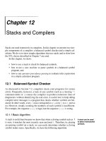
Figure 8.3: Example of a heap storing 13 elements. Each element is a key-value

pair of the form (k, v). The heap is ordered based on the key value, k, of each
element.

Caution

implements the less-than operator between two keys. Suppose that we had instead
defined our comparator to indicate the opposite of the standard total order relation
between keys (so that, for example, isLess(x, y) would return true if x were greater
than y). Then the root of the resulting heap would store the largest key. This
versatility comes essentially for free from our use of the comparator pattern. By
defining the minimum key in terms of the comparator, the “minimum” key with
a “reverse” comparator is in fact the largest. Thus, without loss of generality, we
assume that we are always interested in the minimum key, which is always at the
root of the heap.
For the sake of efficiency, which becomes clear later, we want the heap T to
have as small a height as possible. We enforce this desire by insisting that the heap
T satisfy an additional structural property, it must be complete. Before we define
this structural property, we need some definitions. We recall from Section 7.3.3
that level i of a binary tree T is the set of nodes of T that have depth i. Given nodes
v and w on the same level of T , we say that v is to the left of w if v is encountered
before w in an inorder traversal of T . That is, there is a node u of T such that v is
in the left subtree of u and w is in the right subtree of u. For example, in the binary
tree of Figure 8.3, the node storing entry (15, K) is to the left of the node storing
entry (7, Q). In a standard drawing of a binary tree, the “to the left of” relation is
visualized by the relative horizontal placement of the nodes.
Complete Binary Tree Property: A heap T with height h is a complete binary
tree, that is, levels 0, 1, 2, . . . , h − 1 of T have the maximum number of nodes
possible (namely, level i has 2i nodes, for 0 ≤ i ≤ h − 1) and the nodes at
level h fill this level from left to right.

✐

✐
✐

✐


✐

✐

“main” — 2011/1/13 — 9:10 — page 339 — #361
✐

✐

8.3. Heaps

339

The Height of a Heap
Let h denote the height of T . Another way of defining the last node of T is that
it is the node on level h such that all the other nodes of level h are to the left of
it. Insisting that T be complete also has an important consequence as shown in
Proposition 8.5.
Proposition 8.5: A heap T storing n entries has height
h = ⌊log n⌋.
Justification: From the fact that T is complete, we know that there are 2i nodes
in level, i for 0 ≤ i ≤ h − 1, and level h has at least 1 node. Thus, the number of

nodes of T is at least
(1 + 2 + 4 + · · · + 2h−1 ) + 1 = (2h − 1) + 1
= 2h .
Level h has at most 2h nodes, and thus the number of nodes of T is at most
(1 + 2 + 4 + · · · + 2h−1 ) + 2h = 2h+1 − 1.
Since the number of nodes is equal to the number n of entries, we obtain
2h ≤ n
and

n ≤ 2h+1 − 1.

Thus, by taking logarithms of both sides of these two inequalities, we see that
h ≤ log n
and
log(n + 1) − 1 ≤ h.

Since h is an integer, the two inequalities above imply that
h = ⌊log n⌋.
Proposition 8.5 has an important consequence. It implies that if we can perform
update operations on a heap in time proportional to its height, then those operations
will run in logarithmic time. Therefore, let us turn to the problem of how to efficiently perform various priority queue functions using a heap.

✐

✐
✐

✐

✐

✐

“main” — 2011/1/13 — 9:10 — page 340 — #362
✐

✐

Chapter 8. Heaps and Priority Queues

340

8.3.2 Complete Binary Trees and Their Representation
Let us discuss more about complete binary trees and how they are represented.

The Complete Binary Tree ADT
As an abstract data type, a complete binary tree T supports all the functions of the
binary tree ADT (Section 7.3.1), plus the following two functions:
add(e): Add to T and return a new external node v storing element e, such that the resulting tree is a complete binary
tree with last node v.
remove(): Remove the last node of T and return its element.
By using only these update operations, the resulting tree is guaranteed to be a complete binary. As shown in Figure 8.4, there are essentially two cases for the effect
of an add (and remove is similar).
• If the bottom level of T is not full, then add inserts a new node on the bottom
level of T , immediately after the rightmost node of this level (that is, the last
node); hence, T ’s height remains the same.
• If the bottom level is full, then add inserts a new node as the left child of the
leftmost node of the bottom level of T ; hence, T ’s height increases by one.

w

(a)

(b)

w

(c)

(d)

Figure 8.4: Examples of operations add and remove on a complete binary tree,

where w denotes the node inserted by add or deleted by remove. The trees shown
in (b) and (d) are the results of performing add operations on the trees in (a) and (c),
respectively. Likewise, the trees shown in (a) and (c) are the results of performing
remove operations on the trees in (b) and (d), respectively.

✐

✐
✐

✐


✐

✐

“main” — 2011/1/13 — 9:10 — page 341 — #363
✐

✐

8.3. Heaps

341

A Vector Representation of a Complete Binary Tree
The vector-based binary tree representation (recall Section 7.3.5) is especially suitable for a complete binary tree T . We recall that in this implementation, the nodes
of T are stored in a vector A such that node v in T is the element of A with index
equal to the level number f (v) defined as follows:
• If v is the root of T , then f (v) = 1
• If v is the left child of node u, then f (v) = 2 f (u)
• If v is the right child of node u, then f (v) = 2 f (u) + 1
With this implementation, the nodes of T have contiguous indices in the range [1, n]
and the last node of T is always at index n, where n is the number of nodes of T .
Figure 8.5 shows two examples illustrating this property of the last node.

w
w

(a)

(b)

0 1 2 3 4 5 6

0 1 2 3 4 5 6 7 8

(c)

w

(d)

w

Figure 8.5: Two examples showing that the last node w of a heap with n nodes

has level number n: (a) heap T1 with more than one node on the bottom level;
(b) heap T2 with one node on the bottom level; (c) vector-based representation
of T1 ; (d) vector-based representation of T2 .
The simplifications that come from representing a complete binary tree T with
a vector aid in the implementation of functions add and remove. Assuming that
no array expansion is necessary, functions add and remove can be performed in
O(1) time because they simply involve adding or removing the last element of the
vector. Moreover, the vector associated with T has n + 1 elements (the element at
index 0 is a placeholder). If we use an extendable array that grows and shrinks
for the implementation of the vector (for example, the STL vector class), the space
used by the vector-based representation of a complete binary tree with n nodes is
O(n) and operations add and remove take O(1) amortized time.

✐

✐
✐

✐


✐

✐

“main” — 2011/1/13 — 9:10 — page 342 — #364
✐

✐

342

Chapter 8. Heaps and Priority Queues

A C++ Implementation of a Complete Binary Tree
We present the complete binary tree ADT as an informal interface, called CompleteTree, in Code Fragment 8.11. As with our other informal interfaces, this is not
a complete C++ class. It just gives the public portion of the class.
The interface defines a nested class, called Position, which represents a node of
the tree. We provide the necessary functions to access the root and last positions and
to navigate through the tree. The modifier functions add and remove are provided,
along with a function swap, which swaps the contents of two given nodes.
template <typename E>
class CompleteTree {
// left-complete tree interface
public:
// publicly accessible types
class Position;
// node position type

int size() const;
// number of elements
Position left(const Position& p);
// get left child
Position right(const Position& p);
// get right child
Position parent(const Position& p);
// get parent
bool hasLeft(const Position& p) const; // does node have left child?
bool hasRight(const Position& p) const; // does node have right child?
bool isRoot(const Position& p) const;
// is this the root?
Position root();
// get root position
Position last();
// get last node
void addLast(const E& e);
// add a new last node
void removeLast();
// remove the last node
void swap(const Position& p, const Position& q); // swap node contents
};

Code Fragment 8.11: Interface CompleteBinaryTree for a complete binary tree.

In order to implement this interface, we store the elements in an STL vector,
called V . We implement a tree position as an iterator to this vector. To convert from
the index representation of a node to this positional representation, we provide a
function pos. The reverse conversion is provided by function idx. This portion of
the class definition is given in Code Fragment 8.12.

private:
// member data
std::vector<E> V;
// tree contents
public:
// publicly accessible types
typedef typename std::vector<E>::iterator Position; // a position in the tree
protected:
// protected utility functions
Position pos(int i)
// map an index to a position
{ return V.begin() + i; }
int idx(const Position& p) const
// map a position to an index
{ return p − V.begin(); }
Code Fragment 8.12: Member data and private utilities for a complete tree class.

✐

✐
✐

✐


✐

✐

“main” — 2011/1/13 — 9:10 — page 343 — #365

✐

✐

8.3. Heaps

343

Given the index of a node i, the function pos maps it to a position by adding
i to V.begin(). Here we are exploiting the fact that the STL vector supports a
random-access iterator (recall Section 6.2.5). In particular, given an integer i, the
expression V.begin() + i yields the position of the ith element of the vector, and,
given a position p, the expression p −V.begin() yields the index of position p.
We present a full implementation of a vector-based complete tree ADT in Code
Fragment 8.13. Because the class consists of a large number of small one-line
functions, we have chosen to violate our normal coding conventions by placing all
the function definitions inside the class definition.
template <typename E>
class VectorCompleteTree {
//. . . insert private member data and protected utilities here
public:
VectorCompleteTree() : V(1) {}
// constructor
int size() const
{ return V.size() − 1; }
Position left(const Position& p)
{ return pos(2*idx(p)); }
Position right(const Position& p)
{ return pos(2*idx(p) + 1); }
Position parent(const Position& p)

{ return pos(idx(p)/2); }
bool hasLeft(const Position& p) const
{ return 2*idx(p) <= size(); }
bool hasRight(const Position& p) const { return 2*idx(p) + 1 <= size(); }
bool isRoot(const Position& p) const
{ return idx(p) == 1; }
Position root()
{ return pos(1); }
Position last()
{ return pos(size()); }
void addLast(const E& e)
{ V.push back(e); }
void removeLast()
{ V.pop back(); }
void swap(const Position& p, const Position& q)
{ E e = *q; *q = *p; *p = e; }
};

Code Fragment 8.13: A vector-based implementation of the complete tree ADT.

Recall from Section 7.3.5 that the root node is at index 1 of the vector. Since
STL vectors are indexed starting at 0, our constructor creates the initial vector with
one element. This element at index 0 is never used. As a consequence, the size of
the priority queue is one less than the size of the vector.
Recall from Section 7.3.5 that, given a node at index i, its left and right children
are located at indices 2i and 2i + 1, respectively. Its parent is located at index ⌊i/2⌋.
Given a position p, the functions left, right, and parent first convert p to an index
using the utility idx, which is followed by the appropriate arithmetic operation on
this index, and finally they convert the index back to a position using the utility pos.
We determine whether a node has a child by evaluating the index of this child

and testing whether the node at that index exists in the vector. Operations add
and remove are implemented by adding or removing the last entry of the vector,
respectively.

✐

✐
✐

✐


✐

✐

“main” — 2011/1/13 — 9:10 — page 344 — #366
✐

✐

Chapter 8. Heaps and Priority Queues

344

8.3.3 Implementing a Priority Queue with a Heap
We now discuss how to implement a priority queue using a heap. Our heap-based
representation for a priority queue P consists of the following (see Figure 8.6):
• heap: A complete binary tree T whose nodes store the elements of the queue
and whose keys satisfy the heap-order property. We assume the binary tree T

is implemented using a vector, as described in Section 8.3.2. For each node
v of T , we denote the associated key by k(v).
• comp: A comparator that defines the total order relation among the keys.

Figure 8.6: Illustration of the heap-based implementation of a priority queue.

With this data structure, functions size and empty take O(1) time, as usual. In
addition, function min can also be easily performed in O(1) time by accessing the
entry stored at the root of the heap (which is at index 1 in the vector).

Insertion
Let us consider how to perform insert on a priority queue implemented with a
heap T . To store a new element e in T , we add a new node z to T with operation add,
so that this new node becomes the last node of T , and then store e in this node.
After this action, the tree T is complete, but it may violate the heap-order property. Hence, unless node z is the root of T (that is, the priority queue was empty
before the insertion), we compare key k(z) with the key k(u) stored at the parent
u of z. If k(z) ≥ k(u), the heap-order property is satisfied and the algorithm terminates. If instead k(z) < k(u), then we need to restore the heap-order property,
which can be locally achieved by swapping the entries stored at z and u. (See Figures 8.7(c) and (d).) This swap causes the new entry (k, e) to move up one level.
Again, the heap-order property may be violated, and we continue swapping, going

✐

✐
✐

✐


✐

✐

“main” — 2011/1/13 — 9:10 — page 345 — #367
✐

✐

8.3. Heaps

345

(a)

(b)

(c)

(d)

(e)

(f)

(g)

(h)

Figure 8.7: Insertion of a new entry with key 2 into the heap of Figure8.6: (a) initial

heap; (b) after performing operation add; (c) and (d) swap to locally restore the

partial order property; (e) and (f) another swap; (g) and (h)final swap.

✐

✐
✐

✐