Credit risk modeling using excel and VBA 2 edition

P1: TIX
fm
JWBK493-L¨offler

November 15, 2010

17:8

Printer: Yet to come

Credit Risk Modeling Using Excel
and VBA with DVD

i


P1: TIX
fm
JWBK493-L¨offler

November 15, 2010

17:8

Printer: Yet to come

For other titles in the Wiley Finance series
please see www.wiley.com/finance

ii

P1: TIX
fm
JWBK493-L¨offler

November 15, 2010

17:8

Printer: Yet to come

Credit Risk Modeling Using Excel
and VBA with DVD

Gunter L¨offler
Peter N. Posch

A John Wiley and Sons, Ltd., Publication

iii


P1: TIX
fm
JWBK493-L¨offler

November 15, 2010

17:8

Printer: Yet to come

This edition first published 2011
C 2011 John Wiley & Sons, Ltd
Registered office
John Wiley & Sons Ltd, The Atrium, Southern Gate, Chichester, West Sussex, PO19 8SQ, United Kingdom
For details of our global editorial offices, for customer services and for information about how to apply for
permission to reuse the copyright material in this book please see our website at www.wiley.com.
The right of the author to be identified as the author of this work has been asserted in accordance with the
Copyright, Designs and Patents Act 1988.
All rights reserved. No part of this publication may be reproduced, stored in a retrieval system, or transmitted, in
any form or by any means, electronic, mechanical, photocopying, recording or otherwise, except as permitted by the
UK Copyright, Designs and Patents Act 1988, without the prior permission of the publisher.
Wiley also publishes its books in a variety of electronic formats. Some content that appears in print may not be
available in electronic books.
Designations used by companies to distinguish their products are often claimed as trademarks. All brand names and
product names used in this book are trade names, service marks, trademarks or registered trademarks of their
respective owners. The publisher is not associated with any product or vendor mentioned in this book. This
publication is designed to provide accurate and authoritative information in regard to the subject matter covered. It
is sold on the understanding that the publisher is not engaged in rendering professional services. If professional
advice or other expert assistance is required, the services of a competent professional should be sought.

ISBN 978-0-470-66092-8
A catalogue record for this book is available from the British Library.
Typeset in 10/12pt Times by Aptara Inc., New Delhi, India
Printed in Great Britain by CPI Antony Rowe, Chippenham, Wiltshire

iv

P1: TIX
fm
JWBK493-L¨offler

November 15, 2010

17:8

Printer: Yet to come

Mundus est is qui constat ex caelo, et terra et mare cunctisque sideribus.
Isidoro de Sevilla

v


P1: TIX
fm
JWBK493-L¨offler

November 15, 2010

17:8

Printer: Yet to come

Contents
Preface to the 2nd edition

xi

Preface to the 1st edition

xiii

Some Hints for Troubleshooting

xv

1 Estimating Credit Scores with Logit

1
1
4
8
10
12
16
20
25
25
25
25
26

Linking scores, default probabilities and observed default behavior
Estimating logit coefficients in Excel
Computing statistics after model estimation
Interpreting regression statistics

Prediction and scenario analysis
Treating outliers in input variables
Choosing the functional relationship between the score and explanatory variables
Concluding remarks
Appendix
Logit and probit
Marginal effects
Notes and literature

2 The Structural Approach to Default Prediction and Valuation
Default and valuation in a structural model
Implementing the Merton model with a one-year horizon
The iterative approach
A solution using equity values and equity volatilities
Implementing the Merton model with a T -year horizon
Credit spreads
CreditGrades
Appendix
Notes and literature
Assumptions
Literature

vii

27
27
30
30
35
39

43
44
50
52
52
53


P1: TIX
fm
JWBK493-L¨offler

viii

November 15, 2010

17:8

Printer: Yet to come

Contents

3 Transition Matrices
Cohort approach
Multi-period transitions
Hazard rate approach
Obtaining a generator matrix from a given transition matrix
Confidence intervals with the binomial distribution
Bootstrapped confidence intervals for the hazard approach
Notes and literature

Appendix
Matrix functions

4 Prediction of Default and Transition Rates
Candidate variables for prediction
Predicting investment-grade default rates with linear regression
Predicting investment-grade default rates with Poisson regression
Backtesting the prediction models
Predicting transition matrices
Adjusting transition matrices
Representing transition matrices with a single parameter
Shifting the transition matrix
Backtesting the transition forecasts
Scope of application
Notes and literature
Appendix

5 Prediction of Loss Given Default
Candidate variables for prediction
Instrument-related variables
Firm-specific variables
Macroeconomic variables
Industry variables
Creating a data set
Regression analysis of LGD
Backtesting predictions
Notes and literature
Appendix

55

56
61
63
69
71
74
78
78
78
83
83
85
88
94
99
100
101
103
108
108
110
110
115
115
116
117
118
118
119
120

123
126
126

6 Modeling and Estimating Default Correlations with the Asset
Value Approach
Default correlation, joint default probabilities and the asset value approach
Calibrating the asset value approach to default experience: the method of
moments
Estimating asset correlation with maximum likelihood
Exploring the reliability of estimators with a Monte Carlo study
Concluding remarks
Notes and literature

131
131
133
136
144
147
147


P1: TIX
fm
JWBK493-L¨offler

November 15, 2010

17:8

Printer: Yet to come

Contents

7 Measuring Credit Portfolio Risk with the Asset Value Approach
A default-mode model implemented in the spreadsheet
VBA implementation of a default-mode model
Importance sampling
Quasi Monte Carlo
Assessing Simulation Error
Exploiting portfolio structure in the VBA program
Dealing with parameter uncertainty
Extensions
First extension: Multi-factor model
Second extension: t-distributed asset values
Third extension: Random LGDs
Fourth extension: Other risk measures
Fifth extension: Multi-state modeling
Notes and literature

8 Validation of Rating Systems
Cumulative accuracy profile and accuracy ratios
Receiver operating characteristic (ROC)
Bootstrapping confidence intervals for the accuracy ratio
Interpreting caps and ROCs
Brier score
Testing the calibration of rating-specific default probabilities
Validation strategies
Testing for missing information

Notes and literature

9 Validation of Credit Portfolio Models
Testing distributions with the Berkowitz test
Example implementation of the Berkowitz test
Representing the loss distribution
Simulating the critical chi-square value
Testing modeling details: Berkowitz on subportfolios
Assessing power
Scope and limits of the test
Notes and literature

10 Credit Default Swaps and Risk-Neutral Default Probabilities
Describing the term structure of default: PDs cumulative, marginal and seen
from today
From bond prices to risk-neutral default probabilities
Concepts and formulae
Implementation
Pricing a CDS
Refining the PD estimation

ix

149
149
152
156
160
162
165

168
170
170
171
173
175
177
179
181
182
185
187
190
191
192
195
198
201
203
203
206
207
209
211
214
216
217
219
220
221

221
225
232
234


P1: TIX
fm
JWBK493-L¨offler

x

November 15, 2010

17:8

Printer: Yet to come

Contents

Market values for a CDS
Example
Estimating upfront CDS and the ‘Big Bang’ protocol
Pricing of a pro-rata basket
Forward CDS spreads
Example
Pricing of swaptions
Notes and literature
Appendix
Deriving the hazard rate for a CDS

237
239
240
241
242
243
243
247
247
247

11 Risk Analysis and Pricing of Structured Credit: CDOs and First-to-Default
Swaps
Estimating CDO risk with Monte Carlo simulation
The large homogeneous portfolio (LHP) approximation
Systemic risk of CDO tranches
Default times for first-to-default swaps
CDO pricing in the LHP framework
Simulation-based CDO pricing
Notes and literature
Appendix
Closed-form solution for the LHP model
Cholesky decomposition
Estimating PD structure from a CDS

12 Basel II and Internal Ratings
Calculating capital requirements in the Internal Ratings-Based (IRB) approach
Assessing a given grading structure
Towards an optimal grading structure

Notes and literature

249
249
253
256
259
263
272
281
282
282
283
284
285
285
288
294
297

Appendix A1 Visual Basics for Applications (VBA)

299

Appendix A2 Solver

307

Appendix A3 Maximum Likelihood Estimation and Newton’s Method

313

Appendix A4 Testing and Goodness of Fit

319

Appendix A5 User-defined Functions

325

Index

333


P1: TIX
fm
JWBK493-L¨offler

November 15, 2010

17:8

Printer: Yet to come

Preface to the 2nd Edition
It is common to blame the inadequacy of risk models for the fact that the 2007–2008 financial
crisis caught many market participants by surprise. On closer inspection, though, it often
appears that it was not the models that failed. A good example is the risk contained in
structured finance securities such as collateralized debt obligations (CDOs). In the first edition

of this book, which was published before the crisis, we already pointed out that the rating
of such products is not meant to communicate their systematic risk even though this risk
component can be extremely large. This is easy to illustrate with simple, standard credit risk
models, and surely we were not the first to point this out. Hence, in terms of risk, an AAA-rated
bond is definitely not the same as an AAA-rated CDO. Many institutions, however, appear to
have built their investment strategy on the presumption that AAA is AAA regardless of the
product.
Recent events therefore do not invalidate traditional credit risk modeling as described in
the first edition of the book. A second edition is timely, however, because the first edition
dealt relatively briefly with the pricing of instruments that featured prominently in the crisis
(CDSs and CDOs). In addition to expanding the coverage of these instruments, we devote
more time to modeling aspects that were of particular relevance in the financial crisis (e.g.,
estimation error). We also examine the usefulness and limitations of credit risk modeling
through case studies. For example, we discuss the role of scoring models in the subprime
market, or show that a structural default prediction model would have assigned relatively high
default probabilities to Lehman Brothers in the months before its collapse. Furthermore, we
added a new chapter in which we show how to predict borrower-specific loss given default.
For university teachers, we now offer a set of powerpoint slides as well as problem sets with
solutions. The material can be accessed via our homepage www.loeffler-posch.com.
The hybrid character of the book – introduction to credit risk modeling as well as cookbook for
model implementation – makes it a good companion to a credit risk course, at both introductory
or advanced levels.
We are very grateful to Roger Bowden, Michael Kunisch and Alina Maurer for their
comments on new parts of the book. One of us (Peter) benefited from discussions with a lot of
people in the credit market, among them Nick Atkinson, David Kupfer and Marion Schlicker.
Georg Haas taught him everything a trader needs to know, and Josef Gruber provided him
with valuable insights to the practice of risk management. Several readers of the first edition
pointed out errors or potential for improvement. We would like to use this opportunity to

xi

P1: TIX
fm
JWBK493-L¨offler

xii

November 15, 2010

17:8

Printer: Yet to come

Preface to the 2nd Edition

thank them again and to encourage readers of the second edition to send us their comments
(email: ). Finally, special thanks to our team at Wiley:
Andrew Finch, Brian Burge and our editors Aimee Dibbens and Karen Weller.
At the time of writing it is June. The weather is fine. We are looking forward to devoting
more time to our families again.


P1: TIX
fm
JWBK493-L¨offler

November 15, 2010

17:8

Printer: Yet to come

Preface to the 1st Edition
This book is an introduction to modern credit risk methodology as well as a cookbook for
putting credit risk models to work. We hope that the two purposes go together well. From our
own experience, analytical methods are best understood by implementing them.
Credit risk literature broadly falls into two separate camps: risk measurement and pricing.
We belong to the risk measurement camp. Chapters on default probability estimation and
credit portfolio risk dominate chapters on pricing and credit derivatives. Our coverage of
risk measurement issues is also somewhat selective. We thought it better to be selective than
to include more topics with less detail, hoping that the presented material serves as a good
preparation for tackling other problems not covered in the book.
We have chosen Excel as our primary tool because it is a universal and very flexible tool
that offers elegant solutions to many problems. Even Excel freaks may admit that it is not their
first choice for some problems. But even then, it is nonetheless great for demonstrating how
to put models to work, given that implementation strategies are mostly transferable to other
programming environments. While we tried to provide efficient and general solutions, this
was not our single overriding goal. With the dual purpose of our book in mind, we sometimes
favored a solution that appeared more simple to grasp.
Readers surely benefit from some prior Excel literacy, e.g., knowing how to use a
simple function such as AVERAGE(), being aware of the difference between SUM(A1:A10)
SUM($A1:$A10) and so forth. For less experienced readers, there is an Excel for beginners
video on the DVD, and an introduction to VBA in the Appendix; the other videos supplied on
the DVD should also be very useful as they provide a step-by-step guide more detailed than
the explanations in the main text.
We also assume that the reader is somehow familiar with concepts from elementary statistics
(e.g., probability distributions) and financial economics (e.g., discounting, options). Nevertheless, we explain basic concepts when we think that at least some readers might benefit from
it. For example, we include appendices on maximum likelihood estimation or regressions.
We are very grateful to colleagues, friends and students who gave feedback on the

manuscript: Oliver Bl¨umke, J¨urgen Bohrmann, Andr´e G¨uttler, Florian Kramer, Michael Kunisch, Clemens Prestele, Peter Raupach, Daniel Smith (who also did the narration of the videos
with great dedication) and Thomas Verchow. An anonymous reviewer also provided a lot of
helpful comments. We thank Eva Nacca for formatting work and typing video text. Finally,
we thank our editors Caitlin Cornish, Emily Pears and Vivienne Wickham.

xiii


P1: TIX
fm
JWBK493-L¨offler

xiv

November 15, 2010

17:8

Printer: Yet to come

Preface to the 1st Edition

Any errors and unintentional deviations from best practice remain our own responsibility.
We welcome your comments and suggestions: just send an email to or visit our homepage at www.loeffler-posch.com.
We owe a lot to our families. Before struggling to find the right words to express our
gratitude we rather stop and give our families what they missed most, our time.


P1: TIX
fm

JWBK493-L¨offler

November 15, 2010

17:8

Printer: Yet to come

Some Hints for Troubleshooting
We hope that you do not encounter problems when working with the spreadsheets, macros and
functions developed in this book. If you do, you may want to consider the following possible
reasons for trouble:
We repeatedly use the Excel Solver. This may cause problems if the Solver Add-in is not
activated in Excel and VBA. How this can be done is described in Appendix A2. Apparently,
differences in Excel versions can also lead to situations in which a macro calling the Solver
does not run even though the reference to the Solver is set.
In Chapters 10 and 11, we use functions from the AnalysisToolpak Add-in. Again, this has
to be activated. See Chapter 10 for details.
Some Excel 2003 functions (e.g., BINOMDIST or CRITBINOM) have been changed
relative to earlier Excel versions. We’ve tested our programs on Excel 2003 and Excel
2010. If you’re using an older Excel version, these functions might return error values in
some cases.
All functions have been tested for the demonstrated purpose only. We have not strived to
make them so general that they work for most purposes one can think of. For example:
some functions assume that the data is sorted in some way, or arranged in columns rather
than in rows;
some functions assume that the argument is a range, not an array. See Appendix A1 for
detailed instructions on troubleshooting this issue.
A comprehensive list of all functions (Excel’s and user-defined) together with full syntax
and a short description can be found in Appendix A5.

xv


P1: TIX
c01
JWBK493-L¨offler

November 9, 2010

9:46

Printer: Yet to come

1
Estimating Credit Scores with Logit
Typically, several factors can affect a borrower’s default probability. In the retail segment,
one would consider salary, occupation and other characteristics of the loan applicant; when
dealing with corporate clients, one would examine the firm’s leverage, profitability or cash
flows, to name but a few items. A scoring model specifies how to combine the different pieces
of information in order to get an accurate assessment of default probability, thus serving to
automate and standardize the evaluation of default risk within a financial institution.
In this chapter, we show how to specify a scoring model using a statistical technique called
logistic regression or simply logit. Essentially, this amounts to coding information into a
specific value (e.g., measuring leverage as debt/assets) and then finding the combination of
factors that does the best job in explaining historical default behavior.
After clarifying the link between scores and default probability, we show how to estimate
and interpret a logit model. We then discuss important issues that arise in practical applications,
namely the treatment of outliers and the choice of functional relationship between variables
and default.

An important step in building and running a successful scoring model is its validation. Since
validation techniques are applied not just to scoring models but also to agency ratings and
other measures of default risk, they are described separately in Chapter 8.

LINKING SCORES, DEFAULT PROBABILITIES AND OBSERVED
DEFAULT BEHAVIOR
A score summarizes the information contained in factors that affect default probability. Standard scoring models take the most straightforward approach by linearly combining those
factors. Let x denote the factors (their number is K) and b the weights (or coefficients) attached
to them; we can represent the score that we get in scoring instance i as
Scorei

b1 xi1

b2 xi2

b K xi K

(1.1)

It is convenient to have a shortcut for this expression. Collecting the bs and the xs in column
vectors b and x we can rewrite (1.1) to

Scorei

b1 xi1

b2 xi2

b K xi K

b xi

xi

xi1
xi2
xi K

If the model is to include a constant b1 , we set xi1

b

b1
b2
bK

(1.2)


P1: TIX
c01
JWBK493-L¨offler

2

November 9, 2010

9:46

Printer: Yet to come

Credit Risk Modeling Using Excel and VBA with DVD
Table 1.1 Factor values and default behavior
Default indicator for year

1

Factor values from the end of
year

Scoring instance i

Firm

Year

yi

xi1

xi2

xiK

1
2
3
4

XAX

YOX
TUR
BOK

2001
2001
2001
2001

0
0
0
1

0.12
0.15
0.10
0.16

0.35
0.51
0.63
0.21

0.14
0.04
0.06
0.12

912

913
914

XAX
YOX
TUR

2002
2002
2002

0
0
1

0.01
0.15
0.08

0.02
0.54
0.64

0.09
0.08
0.04

N

VRA

2005

0

0.04

0.76

0.03

behavior.1 Imagine that we have collected annual data on firms with factor values and default
behavior. We show such a data set in Table 1.1.2
Note that the same firm can show up more than once if there is information on this firm for
several years. Upon defaulting, firms often stay in default for several years; in such cases, we
would not use the observations following the year in which default occurred. If a firm moves
out of default, we would again include it in the data set.
The default information is stored in the variable yi . It takes the value 1 if the firm defaulted
in the year following the one for which we have collected the factor values, and zero otherwise.
N denotes the overall number of observations.
The scoring model should predict a high default probability for those observations that
defaulted and a low default probability for those that did not. In order to choose the appropriate
weights b, we first need to link scores to default probabilities. This can be done by representing
default probabilities as a function F of scores:
Prob(Defaulti )

Prob(yi

1)

F(Scorei )

(1.3)

Like default probabilities, the function F should be constrained to the interval from zero to
one; it should also yield a default probability for each possible score. The requirements can be
fulfilled by a cumulative probability distribution function, and a distribution often considered
for this purpose is the logistic distribution. The logistic distribution function (z) is defined
as (z) exp(z) (1 exp(z)). Applied to (1.3) we get
Prob(Defaulti )

(Scorei )

exp(b xi )
1 exp(b xi )

1

1
exp( b xi )

(1.4)

Models that link information to probabilities using the logistic distribution function are called
logit models.
1

In qualitative scoring models, however, experts determine the weights.
Data used for scoring are usually on an annual basis, but one can also choose other frequencies for data collection as well as other
horizons for the default horizon.

2


P1: TIX
c01
JWBK493-L¨offler

November 9, 2010

9:46

Printer: Yet to come

Estimating Credit Scores with Logit

3

Table 1.2 Scores and default probabilities in the logit model

G

H

Prob(Default)

1
2
3
4
5

6
7
8
9
10
11
12
13
14
15
16
17
18

A
B
C
D
E
F
Score Prob(Default)
-8
0.03% =1/(1+EXP(-A2))
-7
0.09% (can be copied into B3:B18)
-6
0 . 25 %
-5
0 . 67 %
100%

-4
1 . 80 %
80%
-3
4 . 74 %
-2
11.92%
60%
-1
26.89%
40%
0
50.00%
1
73.11%
20%
2
88.08%
0%
3
95.26%
-8
-6
-4
-2
0
2
4
98.20%
Score

5
99.33%
6
99.75%
7
99.91%
8
99.97%

4

6

8

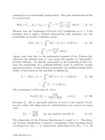
In Table 1.2, we list the default probabilities associated with some score values and illustrate
the relationship with a graph. As can be seen, higher scores correspond to a higher default
probability. In many financial institutions, credit scores have the opposite property: they are
higher for borrowers with a lower credit risk. In addition, they are often constrained to some
set interval, e.g., zero to 100. Preferences for such characteristics can easily be met. If we use
(1.4) to define a scoring system with scores from 9 to 1, but want to work with scores from
0 to 100 instead (100 being the best), we could transform the original score to myscore
10 score 10.
Having collected the factors x and chosen the distribution function F, a natural way of
estimating the weights b is the maximum likelihood (ML) method. According to the ML
principle, the weights are chosen such that the probability ( likelihood) of observing the
given default behavior is maximized (see Appendix A3 for further details on ML estimation).
The first step in maximum likelihood estimation is to set up the likelihood function. For a
borrower that defaulted, the likelihood of observing this is
Prob(Defaulti )

Prob(yi

1)

(b xi )

(1.5)

For a borrower that did not default, we get the likelihood
Prob(No defaulti )

Prob(yi

0)

1

(b xi )

(1.6)

Using a little trick, we can combine the two formulae into one that automatically gives
the correct likelihood, be it a defaulter or not. Since any number raised to the power of zero


P1: TIX
c01
JWBK493-L¨offler

4

November 9, 2010

9:46

Printer: Yet to come

Credit Risk Modeling Using Excel and VBA with DVD

evaluates to one, the likelihood for observation i can be written as
( (b xi )) yi (1

Li

(b xi ))1

yi

(1.7)

Assuming that defaults are independent, the likelihood of a set of observations is just the
product of the individual likelihoods:3
N

N

L

( (b xi )) yi (1

Li
i 1

(b xi ))1

yi

(1.8)

i 1

For the purpose of maximization, it is more convenient to examine ln L, the logarithm of
the likelihood:
N

ln L

yi ln( (b xi ))

(1

yi ) ln(1

(b xi ))

(1.9)

i 1

It can be maximized by setting its first derivative with respect to b to zero. This derivative
(like b, it is a vector) is given by
N

ln L
b

(yi

(b xi ))xi

(1.10)

i 1

Newton’s method (see Appendix A3) does a very good job in solving equation (1.10) with
respect to b. To apply this method, we also need the second derivative, which we obtain as
2

ln L
b b

N

(b xi )(1

(b xi ))xi xi

(1.11)

i 1

ESTIMATING LOGIT COEFFICIENTS IN EXCEL
Excel does not contain a function for estimating logit models, and so we sketch how to
construct a user-defined function that performs the task. Our complete function is called
LOGIT. The syntax of the LOGIT command is equivalent to the LINEST command:
LOGIT(y,x,[const],[statistics]), where [] denotes an optional argument.
The first argument specifies the range of the dependent variable, which in our case is the
default indicator y; the second parameter specifies the range of the explanatory variable(s).
The third and fourth parameters are logical values for the inclusion of a constant (1 or omitted
if a constant is included, 0 otherwise) and the calculation of regression statistics (1 if statistics
are to be computed, 0 or omitted otherwise). The function returns an array, therefore, it has to
be executed on a range of cells and entered by [ctrl] [shift] [enter].
3
Given that there are years in which default rates are high, and others in which they are low, one may wonder whether the independence
assumption is appropriate. It will be if the factors that we input into the score capture fluctuations in average default risk. In many
applications, this is a reasonable assumption.


P1: TIX
c01
JWBK493-L¨offler

November 9, 2010

9:46

Printer: Yet to come

Estimating Credit Scores with Logit

5

Table 1.3 Application of the LOGIT command to a data set with information on defaults and five
financial ratios
A

B

C

D

E

F

G

H

Firm
ID

Year

Default

WC/
TA

RE/
TA

EBIT/
TA

ME/
TL

S/
TA

0.31
0.32
0.23
0.19
0.22
0.22
-0.03
-0.12

0.04
0.05
0.03
0.03
0.03
0.03
0.01
0.03

0.96
1.06
0.80
0.39
0.79
1.29
0.11
0.15

1
2
1
3
1
4
1
5
1
6
1
7
1
8
2
9
2
…
108
21

…
4001 830

1999
2000
2001
2002
2003
2004
1999
2000

0
0
0
0
0
0
0
0

0.50
0.55
0.45
0.31
0.45
0.46
0.01
-0.11

0.33
0.33
0.25
0.25
0.28
0.32
0.25
0.32

1996

1

0.36 0.06 0.03 3.20 0.28

2002

1

0.07 -0.11 0.04 0.04 0.12

I
b

J

K

L

M

N

O

CONST

WC/
TA

RE/
TA

EBIT/
TA

ME/
TL

S/
TA

-2.543 0.414 -1.454 -7.999 -1.594 0.620
{=LOGIT(C2:C4001,D2:H4001,1,0)}
(applies to J2:O2)

Before delving into the code, let us look at how the function works on an example data
set.4 We have collected default information and five variables for default prediction; Working
Capital (WC), Retained Earnings (RE), Earnings Before Interest and Taxes (EBIT) and Sales

(S), each divided by Total Assets (TA); and Market Value of Equity (ME) divided by Total
Liabilities (TL). Except for the market value, all these items are found in the balance sheet
and income statement of the company. The market value is given by the number of shares
outstanding multiplied by the stock price. The five ratios are the ones from the widely known
Z-score developed by Altman (1968). WC/TA captures the short-term liquidity of a firm,
RE/TA and EBIT/TA measure historic and current profitability, respectively. S/TA further
proxies for the competitive situation of the company and ME/TL is a market-based measure
of leverage.
Of course, one could consider other variables as well; to mention only a few, these could be:
cash flows over debt service, sales or total assets (as a proxy for size), earnings volatility, stock
price volatility. In addition, there are often several ways of capturing one underlying factor.
Current profits, for instance, can be measured using EBIT, EBITDA ( EBIT plus depreciation
and amortization) or net income.
In Table 1.3, the data is assembled in columns A to H. Firm ID and year are not required
for estimation. The LOGIT function is applied to range J2:O2. The default variable that the
LOGIT function uses is in the range C2:C4001, while the factors x are in the range D2:H4001.
Note that (unlike in Excel’s LINEST function) coefficients are returned in the same order
as the variables are entered; the constant (if included) appears as the leftmost variable. To
interpret the sign of the coefficient b, recall that a higher score corresponds to a higher default
probability. The negative sign of the coefficient for EBIT/TA, for example, means that default
probability goes down as profitability increases.
Now let us have a close look at important parts of the LOGIT code. In the first lines
of the function, we analyze the input data to define the data dimensions: the total number
of observations N and the number of explanatory variables (including the constant) K. If a
4

The data is hypothetical, but mirrors the structure of data for listed US corporates.


P1: TIX

c01
JWBK493-L¨offler

6

November 9, 2010

9:46

Printer: Yet to come

Credit Risk Modeling Using Excel and VBA with DVD

constant is to be included (which should be done routinely) we have to add a vector of 1s to
the matrix of explanatory variables. This is why we call the read-in factors xraw, and use
them to construct the matrix x we work with in the function by adding a vector of 1s. For this,
we could use an If-condition, but here we just write a 1 in the first column and then overwrite
it if necessary (i.e., if constant is zero):
Function LOGIT(y As Range, xraw As Range, _
Optional constant As Byte, Optional stats As Byte)
If IsMissing(constant) Then constant
If IsMissing(stats) Then stats
0

1

'Count variables
Dim i As long, j As long, jj As long
'Read data dimensions
Dim K As Long, N As Long

y.Rows.Count
N
K
xraw.Columns.Count
constant
'Adding a vector of ones to the x matrix if constant 1,
'name xraw x from now on
Dim x() As Double
ReDim x(1 To N, 1 To K)
For i
1 To N
1
x(i, 1)
For j
1
constant To K
x(i, j)
xraw(i, j - constant)
Next j
Next i

The logical value for the constant and the statistics are read in as variables of type byte,
meaning that they can take integer values between 0 and 255. In the function, we could
therefore check whether the user has indeed input either zero or 1, and return an error message
if this is not the case. Both variables are optional, if their input is omitted the constant is
set to 1 and the statistics to 0. Similarly, we might want to send other error messages, e.g.,
if the dimension of the dependent variable y and the one of the independent variables x do
not match.
The way we present it, the LOGIT function requires the input data to be organized in
columns, not in rows. For the estimation of scoring models, this will be standard, because the

number of observations is typically very large. However, we could modify the function in such
a way that it recognizes the organization of the data. The LOGIT function maximizes the loglikelihood by setting its first derivative to zero, and uses Newton’s method (see Appendix A3)
to solve this problem. Required for this process are: a set of starting values for the unknown
parameter vector b; the first derivative of the log-likelihood (the gradient vector g() given in
(1.10)); the second derivative (the Hessian matrix H() given in (1.11)). Newton’s method then


P1: TIX
c01
JWBK493-L¨offler

November 9, 2010

9:46

Printer: Yet to come

Estimating Credit Scores with Logit

7

leads to the following rule:
1

2

b1

ln L
b0 b0

b0

ln L
b0

b0

H (b0 ) 1 g(b0 )

(1.12)

The logit model has the nice feature that the log-likelihood function is globally concave.
Once we have found the root to the first derivative, we can be sure that we have found the
global maximum of the likelihood function.
When initializing the coefficient vector (denoted by b in the function), we can already
initialize the score b x (denoted by bx), which will be needed later on:
'Initializing the coefficient vector (b) and the score (bx)
Dim b() As Double, bx() As Double
ReDim b(1 To K): ReDim bx(1 To N)

Since we only declare the coefficients and the score, their starting values are implicitly
set to zero. Now we are ready to start Newton’s method. The iteration is conducted within a
Do-while loop. We exit once the change in the log-likelihood from one iteration to the next
does not exceed a certain small value (like 10 11 ). Iterations are indexed by the variable iter.
Focusing on the important steps, once we have declared the arrays dlnl (gradient), Lambda
(prediction (b x)), hesse (Hessian matrix) and lnl (log-likelihood), we compute their
values for a given set of coefficients, and therefore for a given score bx. For your convenience,
we summarize the key formulae below the code:
'Compute prediction Lambda, gradient dlnl,

'Hessian hesse, and log likelihood lnl
For i
1 To N
Lambda(i)
1 / (1
Exp(-bx(i)))
1 To K
For j
dlnL(j)
dlnL(j)
(y(i) - Lambda(i)) * x(i, j)
For jj
1 To K
hesse(jj, j) - Lambda(i) * (1 - Lambda(i)) _
hesse(jj, j)
* x(i, jj) * x(i, j)
Next jj
Next j
lnL(iter)
y(i) * Log(Lambda(i))
(1 - y(i)) _
lnL(iter)
* Log(1 - Lambda(i))
Next i

Lambda

(b xi )

1 (1

exp( b xi ))

N

dlnl

(yi

(b xi ))xi

i 1
N

hesse

(b xi )(1

(b xi ))xi xi

i 1
N

lnl

yi ln( (b xi ))
i 1

(1

yi ) ln(1

(b xi ))


P1: TIX
c01
JWBK493-L¨offler

8

November 9, 2010

9:46

Printer: Yet to come

Credit Risk Modeling Using Excel and VBA with DVD

We have to go through three loops. The function for the gradient, the Hessian and the
likelihood each contain a sum for i 1 to N. We use a loop from i 1 to N to evaluate
those sums. Within this loop, we loop through j 1 to K for each element of the gradient
vector; for the Hessian, we need to loop twice, and so there is a second loop jj 1 to K.
Note that the gradient and the Hessian have to be reset to zero before we redo the calculation
in the next step of the iteration.
With the gradient and the Hessian at hand, we can apply Newton’s rule. We take the inverse
of the Hessian using the worksheet-Function MINVERSE, and multiply it with the gradient
using the worksheet-Function MMULT:
'Compute inverse Hessian ( hinv) and multiply hinv with gradient dlnl
Application.WorksheetFunction.MInverse(hesse)

hinv
hinvg
Application.WorksheetFunction.MMult(dlnL, hinv)
sens Then Exit Do
If Abs(change)
' Apply Newton’s scheme for updating coefficients b
For j
1 To K
b(j) - hinvg(j)
b(j)
Next j

As outlined above, this procedure of updating the coefficient vector b is ended when the
change in the likelihood, abs(ln(iter)-ln(iter-1)), is sufficiently small. We can
then forward b to the output of the function LOGIT.

COMPUTING STATISTICS AFTER MODEL ESTIMATION
In this section, we show how the regression statistics are computed in the LOGIT function. Readers wanting to know more about the statistical background may want to consult
Appendix A4.
To assess whether a variable helps explain the default event or not, one can examine a t-ratio
for the hypothesis that the variable’s coefficient is zero. For the jth coefficient, such a t-ratio is
constructed as
tj

b j SE(b j )

(1.13)

where SE is the estimated standard error of the coefficient. We take b from the last iteration
of the Newton scheme and the standard errors of estimated parameters are derived from the

Hessian matrix. Specifically, the variance of the parameter vector is the main diagonal of the
negative inverse of the Hessian at the last iteration step. In the LOGIT function, we have
already computed the Hessian hinv for the Newton iteration, and so we can quickly calculate
the standard errors. We simply set the standard error of the jth coefficient to Sqr(-hinv(j,
j). t-ratios are then computed using Equation (1.13).
In the logit model, the t-ratio does not follow a t-distribution as in the classical linear
regression. Rather, it is compared to a standard normal distribution. To get the p-value of a


P1: TIX
c01
JWBK493-L¨offler

November 9, 2010

9:46

Printer: Yet to come

Estimating Credit Scores with Logit

9

two-sided test, we exploit the symmetry of the normal distribution:
p-value

2 (1-NORMSDIST(ABS(t)))

(1.14)

The LOGIT function returns standard errors, t-ratios and p-values in lines two to four of the
output if the logical value statistics is set to 1.
In a linear regression, we would report an R2 as a measure of the overall goodness of fit.
In nonlinear models estimated with maximum likelihood, one usually reports the Pseudo-R2
suggested by McFadden (1974). It is calculated as 1 minus the ratio of the log-likelihood of
the estimated model (ln L) and the one of a restricted model that has only a constant (ln L0 ):
Pseudo-R 2

1

ln L ln L 0

(1.15)

Like the standard R2 , this measure is bounded by zero and one. Higher values indicate a
better fit. The log-likelihood ln L is given by the log-likelihood function of the last iteration of
the Newton procedure, and is thus already available. Left to determine is the log-likelihood of
the restricted model. With a constant only, the likelihood is maximized if the predicted default
probability is equal to the mean default rate y¯ . This can be achieved by setting the constant
equal to the logit of the default rate, i.e., b1 ln( y¯ (1 y¯ )). For the restricted log-likelihood,
we then obtain:
N

ln L 0

yi ln( (b xi ))

(1

yi ) ln(1

(b xi ))

i 1
N

yi ln( y¯ )

(1

yi ) ln(1

y¯ )

N [ y¯ ln( y¯ )

(1

y¯ ) ln(1

y¯ )]

(1.16)

i 1

In the LOGIT function, this is implemented as follows:
'ln Likelihood of model with just a constant(lnL0)
Dim lnL0 As Double, ybar as Double
ybar

Application.WorksheetFunction.Average(y)
N * (ybar * Log(ybar)
(1 - ybar) * Log(1 - ybar))
lnL0

The two likelihoods used for the Pseudo-R2 can also be used to conduct a statistical test of
the entire model, i.e., test the null hypothesis that all coefficients except for the constant are
zero. The test is structured as a likelihood ratio test:
LR

2(ln L

ln L 0 )

(1.17)

The more likelihood is lost by imposing the restriction, the larger the LR-statistic will be.
The test statistic is distributed asymptotically chi-squared with the degrees of freedom equal to
the number of restrictions imposed. When testing the significance of the entire regression, the
number of restrictions equals the number of variables K minus 1. The function CHIDIST(test
statistic, restrictions) gives the p-value of the LR test. The LOGIT command returns both the
LR and its p-value.


P1: TIX
c01
JWBK493-L¨offler

November 9, 2010

10

9:46

Printer: Yet to come

Credit Risk Modeling Using Excel and VBA with DVD
Table 1.4 Output of the user-defined function LOGIT

b1

b2

bK

SE(b1 )
t1 b1 /SE(b1 )
p-value(t1 )
Pseudo-R2
LR-test
log-likelihood (model)

SE(b2 )
t2 b2 /SE(b2 )
p-value(t2 )
# iterations
p-value (LR)
log-likelihood(restricted)

SE(bK )

tK bK /SE(bK )
p-value(tK )
#N/A
#N/A
#N/A

#N/A
#N/A
#N/A

The likelihoods ln L and ln L0 are also reported, as is the number of iterations that was
needed to achieve convergence. As a summary, the output of the LOGIT function is organized
as shown in Table 1.4.

INTERPRETING REGRESSION STATISTICS
Applying the LOGIT function to our data from Table 1.3 with the logical values for constant
and statistics both set to 1, we obtain the results reported in Table 1.5. Let us start with the
statistics on the overall fit. The LR test (in J7, p-value in K7) implies that the logit regression is
highly significant. The hypothesis ‘the five ratios add nothing to the prediction’ can be rejected
with high confidence. From the three decimal points displayed in Table 1.5, we can deduce
that the significance is better than 0.1%, but in fact it is almost indistinguishable from zero
(being smaller than 10 36 ). So we can trust that the regression model helps explain the default
events.
Knowing that the model does predict defaults, we would like to know how well it does so.
One usually turns to the R2 for answering this question, but as in linear regression, setting up
general quality standards in terms of a Pseudo-R2 is difficult to impossible. A simple but often
effective way of assessing the Pseudo-R2 is to compare it with the ones from other models
Table 1.5 Application of the LOGIT command to a data set with information on defaults and five
financial ratios (with statistics)

1
2
3
4
5
6
7
8
9
…
108
…
4001

C

D

E

F

G

H

Default y

WC/
TA

RE/
TA

EBIT/
TA

ME/
TL

S/
TA

0.50
0.55
0.45
0.31
0.45
0.46
0.01
-0.11
…
0.36
…
0.07

0.31
0.32
0.23
0.19

0.22
0.22
-0.03
-0.12
…
0.06
…
-0.11

0.04
0.05
0.03
0.03
0.03
0.03
0.01
0.03
…
0.03
…
0.04

0.96
1.06
0.80
0.39
0.79
1.29
0.11
0.15

…
3.20
…
0.04

0
0
0
0
0
0
0
0
…
1
…
1

I

J

K

L

M

N

O

CONST

WC/
TA

RE/
TA

EBIT/
TA

ME/
TL

S/
TA

0.33
b -2.543 0.414 -1.454 -7.999 -1.594 0.620
0.33
SE(b) 0.266 0.572 0.229 2.702 0.323 0.349
0.25
t -9.56 0.72 -6.34 -2.96 -4.93 1.77
0.25
p-value 0.000 0.469 0.000 0.003 0.000 0.076
0.28 Pseudo R² / # iter 0.222
12 #N/A #N/A #N/A #N/A
0.32 LR-test / p-value 160.1 0.000 #N/A #N/A #N/A #N/A

0.25
lnL / lnL 0 -280.5 -360.6 #N/A #N/A #N/A #N/A
{=LOGIT(C2:C4001,D2:H4001,1,1)}
0.32
…
(applies to J2:O8)
0.28
…
0.12