Ebook A handbook of applied statistics in pharmacology: Part 1
Bạn đang xem bản rút gọn của tài liệu. Xem và tải ngay bản đầy đủ của tài liệu tại đây (913.14 KB, 120 trang )
A Handbook of
Applied
Statistics in
Pharmacology
Median
Lower Hinge
Upper Hinge
Whisker
Whisker
Hinge Spread
A SCIENCE PUBL
PUBLISHERS
UBLIISHERS BOOK
130
135
140
145
150
155
160
165
170
A Handbook of Applied Statistics
in Pharmacology
A Handbook of Applied Statistics
in Pharmacology
Katsumi Kobayashi
Safety Assessment Division, Chemical Management Center
National Institute of Technology and Evaluation (NITE)
Tokyo, Japan
K. Sadasivan Pillai
Frontier Life Science Services
(A Unit of Frontier Lifeline Hospitals)
Thiruvallur District
Chennai, India
p,
A SCIENCE PUBLISHERS BOOK
CRC Press
Taylor & Francis Group
6000 Broken Sound Parkway NW, Suite 300
Boca Raton, FL 33487-2742
© 2013 by Taylor & Francis Group, LLC
CRC Press is an imprint of Taylor & Francis Group, an Informa business
No claim to original U.S. Government works
Version Date: 2012919
International Standard Book Number-13: 978-1-4665-1540-6 (eBook - PDF)
This book contains information obtained from authentic and highly regarded sources. Reasonable
efforts have been made to publish reliable data and information, but the author and publisher cannot
assume responsibility for the validity of all materials or the consequences of their use. The authors and
publishers have attempted to trace the copyright holders of all material reproduced in this publication
and apologize to copyright holders if permission to publish in this form has not been obtained. If any
copyright material has not been acknowledged please write and let us know so we may rectify in any
future reprint.
Except as permitted under U.S. Copyright Law, no part of this book may be reprinted, reproduced,
transmitted, or utilized in any form by any electronic, mechanical, or other means, now known or
hereafter invented, including photocopying, microfilming, and recording, or in any information storage or retrieval system, without written permission from the publishers.
For permission to photocopy or use material electronically from this work, please access www.copyright.com ( or contact the Copyright Clearance Center, Inc. (CCC), 222
Rosewood Drive, Danvers, MA 01923, 978-750-8400. CCC is a not-for-profit organization that provides licenses and registration for a variety of users. For organizations that have been granted a photocopy license by the CCC, a separate system of payment has been arranged.
Trademark Notice: Product or corporate names may be trademarks or registered trademarks, and are
used only for identification and explanation without intent to infringe.
Visit the Taylor & Francis Web site at
and the CRC Press Web site at
Foreword
Life expectancy has signi¿cantly increased in the last century, thanks to
the discovery and development of new drugs by pharmaceutical industries.
Search for new therapeutics is the primary activity of the R&D of
pharmaceutical industries and it involves complex network of tasks such as
synthetic chemistry, in vitro/in vivo ef¿cacy, safety, preclinical and clinical
research. Statistical analysis has always been the foundation to establish the
safety and ef¿cacy of drugs. The decision to- or not to- advance preclinical
drug candidates to very expensive clinical development heavily relies on
statistical analysis and the resulting signi¿cance of preclinical data. Recent
reports attributed failure of certain drugs in clinical stages of development
to improper conduct of preclinical studies and inappropriate application
of statistical tools. Applying appropriate statistical tools is sagacious
to analysis of data from any research activity. Though scientists expect
computerized statistical packages to perform analyses of the data, he/she
should be familiar with the underlying principles to choose the appropriate
statistical tool.
‘A Handbook of Applied Statistics in Pharmacology’ by Katsumi
Kobayashi and K. Sadasivan Pillai is a very useful book for scientists
working in R&D of pharmaceuticals and contract research organizations.
Most of the routine statistical tools used in pharmacology and toxicology
are covered perspicuously in the book. The examples worked out in the
book are from actual studies, hence do not push a reader having less or no
exposure to statistics outside his/her comfort zone.
Dr. K.M. Cherian
M.S., F.R.A.C.S., Ph.D., D.Sc. (Hon.), D.Sc. (CHC), D.Sc. (HC)
Chairman & CEO
Frontier Lifeline Hospitals
Chennai, India
Preface
Scientists involved in pharmacology have always felt that statistics is a
dif¿cult subject to tackle. Thus they heavily rely on statisticians to analyse
their experimental data. No doubt, statisticians with some scienti¿c
knowledge can analyse the data, but their interpretation of results often
perplexes the scientists.
Statistics play an important role in pharmacology and related subjects
like, toxicology, and drug discovery and development. Improper statistical
tool selection to analyze the data obtained from studies conducted in
these subjects may result in erroneous interpretation of the performanceor safety- of drugs. There have been several incidents in pharmaceutical
industries, where failure of drugs in clinical trials is attributed to improper
statistical analysis of the preclinical data. In pharmaceutical Research
& Development settings, where a large number of new drug entities are
subjected to high-throughput in vitro and in vivo studies, use of appropriate
statistical tools is quintessential.
It is not prudent for the research scientists to totally depend on
statisticians to interpret the ¿ndings of their hard work. Factually, scientists
with basic statistical knowledge and understanding of the underlying
principles of statistical tools selected for analysing the data have an
advantage over others, who shy away from statistics. Underlying principle
of a statistical tool does not mean that one should learn all complicated
mathematical jargons. Here, the underlying principle means only ‘thinking
logically’ or applying ‘common sense’.
The authors of this book, with decades of experience in contract
research organizations and pharmaceutical industries, are fully cognizant
of the extent of literacy in statistics that the research scientists working in
pharmacology, toxicology, and drug discovery and development would be
interested to learn. This book is written with an objective to communicate
statistical tools in simple language. Utmost care has been taken to avoid
complicated mathematical equations, which the readers may ¿nd dif¿cult
viii A Handbook of Applied Statistics in Pharmacology
to assimilate. The examples used in the book are similar to those that the
scientists encounter regularly in their research. The authors have provided
cognitive clues for selection of an appropriate statistical tool to analyse the
data obtained from the studies and also how to interpret the result of the
statistical analysis.
Contents
Foreword
Preface
v
vii
1. Probability
Probability and Possibility
Probability—Examples
Probability Distribution
Cumulative Probability
Probability and Randomization
1
1
2
3
3
4
2. Distribution
History
Variable
Stem-and-Leaf Plot
Box-and-Whisker Plot
6
6
6
7
8
3. Mean, Mode, Median
Average and Mean
Mean
Geometric Mean
Harmonic Mean
Weighted Mean
Mode
Median
11
11
11
12
12
13
13
14
4. Variance, Standard Deviation, Standard Error,
Coef¿cient of Variation
Variance
Standard Deviation (SD)
Standard Error (SE)
Coef¿cient of Variation (CV)
When to Use a Standard Deviation (SD)/Standard Error (SE)?
16
16
18
19
19
20
x
A Handbook of Applied Statistics in Pharmacology
5. Analysis of Normality and Homogeneity of Variance
Distribution of Data in Toxicology and Pharmacology
Experiments
Analysis of Normality
Tests for Analyzing Normal Distribution
Shapiro-Wilk’s W test
Power of Shapiro-Wilk’s W test
Parametric and Non-parametric Analyses
Analysis of Homogeneity of Variance
Bartlett’s homogeneity test
Levene’s homogeneity test
Power of Bartlett’s and Levene’s homogeneity tests
Do We Need to Examine the Data for Both Normality and
Homogeneity?
Which Test to be Used for Examining Homogeneity of Variance?
23
23
33
6. Transformation of Data and Outliers
Transformation of Data
Outliers
Masuyama’s Rejection Limit Test
Thompson’s Rejection Test
Smirnov-Grubbs’ Rejection Test
A Cautionary Note
37
37
38
40
41
42
42
7. Tests for Signi¿cant Differences
Null Hypothesis
Signi¿cant Level, Type I and Type II Errors
Why at 5% Signi¿cant Level?
How to Express P?
One-sided and Two-sided Tests
Which Test to Use: One-sided or Two-sided?
47
47
48
48
50
50
51
8. t-Tests
Student’s t-Test—History
t-Test for One Group
t-Test for Two Groups
Student’s t-test
Aspin-Welch’s t-test
Cochran-Cox’s t-test
Paired t-Test
A Note of Caution
56
56
56
57
58
60
62
64
65
23
24
24
27
31
31
31
32
32
33
Contents
9. Correlation Analysis
Correlation and Association
Pearson’s Product Moment Correlation Coef¿cient
Signi¿cance of r
Con¿dence Interval of Correlation Coef¿cient
Coef¿cient of Determination
Rank Correlation
Spearman’s Rank Correlation
Canonical Correlation
Misuse of Correlation Analysis
10. Regression Analysis
History
Linear Regression Analysis
Con¿dence Limits for Slope
Comparison of Two Regression Coef¿cients
R2
Multiple Linear Regression Analysis
Polynomial Regression
Misuse of Regression Analysis
xi
67
67
68
69
70
71
71
71
72
72
74
74
74
78
79
80
80
81
82
11. Multivariate Analysis
Analysis of More than Two Groups
One-way ANOVA
post hoc Comparison
Dunnett’s multiple comparison test
Tukey’s multiple range test
Williams’s test
Duncan’s multiple range test
Scheffé’s multiple comparison test
Two-way ANOVA
Dunnett’s Multiple Comparison Test and Student’s
t Test—A Comparison
84
84
85
87
87
89
90
95
98
100
103
12. Non-Parametric Tests
Non-parametric and Parametric Tests—Assumptions
Sign Tests
Calculation procedure of sign test for small sample size
Calculation procedure of sign test for large sample size
106
106
106
107
107
xii A Handbook of Applied Statistics in Pharmacology
Signed Rank Sum Tests
Wilcoxon rank-sum test
Fisher’s exact test
Mann-Whitney’s U test
Kruskal-Wallis Nonparametric ANOVA by Ranks
Comparison of Group Means
Dunn’s multiple comparison test for more than three groups
Steel’s multiple comparison test for more than three groups
Rank Sum Tests—Some Points
109
109
111
113
117
119
120
121
123
13. Cluster Analysis
What is Cluster Analysis?
Hierarchical cluster analysis
Ward’s method of cluster analysis
k-means cluster analysis
127
127
127
128
129
14. Trend Tests
Introduction
Jonckheere’s trend test
The Cochran-Armitage test
136
136
136
139
15. Survival Analysis
Introduction
Hazard Rate
Kaplan-Meier Method
Kaplan-Meier product-limit estimator
143
143
144
144
144
16. Dose Response Relationships
Dose and Dosage
Margin of Exposure, NOAEL, NOEL
Determining NOEL and NOAEL
Benchmark Dose
Probit Analysis
IC50 and EC50 Determination
Hormesis
150
150
150
152
153
154
157
158
17. Analysis of Pathology Data
Pathology in Toxicology
Analysis of Pathology Data of Carcinogenicity Studies
Peto test
Decision rules
163
163
164
165
166
Contents
Poly-k Type test
Analysis of Tumour Incidence—Comparison with Historical
Control Data
Analysis of Incidence of Tumour Using X 2 Test
Comparison of Incidence of Tumours in Human, Rats, Mice
and Dogs
Analysis of Organ Weight Data
Interpretation of Pathology Observations
xiii
167
168
170
170
172
173
18. Designing An Animal Experiment in Pharmacology and
Toxicology—Randomization, Determining Sample Size
Designing Animal Experiments
Acclimation
Randomization
Determining Sample Size
Animal Experimental Designs
178
19. How to Select An Appropriate Statistical Tool?
Good Statistical Design
Decision Trees
Statistical Procedures Used by National Toxicology
Program (NTP), USA
Decision Tree Produced by OECD
Incongruence in Selection of a Statistical Tool
Selection of a Statistical Tool—Suggested Decision Trees
or Flow Charts
Statistical Tools Suggested for the Analysis of Toxicology Data
Use of Statistics in Toxicology-Limitations
188
188
188
191
178
179
179
183
185
193
194
195
196
196
Appendices
Appendix 1. Coef¿cient for Shapiro-Wilk W Test
Appendix 2. Quantiles of the Shapiro-Wilk Test Statistic
Appendix 3. Z Score for Normal Distribution
201
202
206
208
Index
211
1
Probability
Probability and Possibility
We all are familiar with the words, possibility and probability. Though
these words seem to convey similar meanings, in reality they do not.
Imagine, your greatest ambition is to climb Mount Everest. But you do
not know the basics of mountaineering and have not climbed even a
hill before. It may still be possible for you to climb Mount Everest, if
you learn mountaineering techniques and undergo strenuous training in
mountaineering. But the probability of accomplishing your ambition of
climbing Mount Everest is remote. Possibility is the event that can happen
in life, whereas the probability is the chance of that happening. In statistical
terminology, an event is collection of results or outcomes of a procedure.
Probability is the basic of statistics.
Mathematicians developed the ‘principle of indifference’ over 300
years ago to elucidate the ‘science of gaming’ (Murphy, 1985). According
to Keynes (1921), the ‘principle of indifference’ asserts that “if there is
no known reason for predicating of our subject one rather than another of
several alternatives, then relatively to such knowledge the assertions of
each of these alternatives have an equal probability.” In other words, if you
have no reason to believe the performance of drug A is better than B, then
you should not believe that drug A is better than B.
The two approaches to probability are classical approach and relative
frequency approach. In classical approach, the number of successful
outcomes is divided by the total number of equally likely outcomes. Relative
frequency is the frequency of an event occurring in large number of trials.
For example, you Àip a coin 1000 times and the number of occurrences of
head up is 520. The probability of head up is 520/1000=0.52.
2
A Handbook of Applied Statistics in Pharmacology
Both the classical and frequency approaches have some drawbacks.
Because of these drawbacks, an axiomatic approach to probability has
been suggested by mathematicians (Spiegel et al., 2002).
However, in pharmacology and toxicology experiments, relative
frequency approach proposed by Mises and Reichenbach (Carnap, 1995)
works well.
We shall understand probability a bit more in detail by working out
examples.
Probability—Examples
Let us try to de¿ne a probability with regard to frequency approach. The
probability of an occurrence for an event labeled A is de¿ned as the ratio of
the number of events where event A occurs to the total number of possible
events that could occur (Selvin, 2004).
Let us understand some basic notations of probability:
P denotes probability.
If you toss a coin, only two events can occur, either a head up or a tail
up.
P(H) denotes probability of event head is up. You can calculate the
probability of head coming up using the formula:
Number of times head is up
P(H) =
(Number of times head is up+Number of times tail is up)
Remember, a head up and a tail up have equal chance of occurring. Ideally
you will get a value very close to 50% for P(H), if you toss the coin several
times.
You roll an unbiased six-sided dice. The total number of outcomes is
six, which are equally likely. This means the likelihood of ‘any number’
coming up is same as ‘any other number’. The probability of any number
coming up is 1/6. The probability of any two numbers coming up is 2/6.
Let us come back to our example of tossing a coin. The probability of
a head up is ½ (0.5 or 50%). Now you Àip the coin twice. The probability
of a head up both times is ½ x ½ = ¼.
Probability
3
Mutually exclusive events
While you toss a coin either a head up or a tail up occurs. When the event
head up occurs, the event tail up cannot occur and vice versa; one event
precludes the occurrence of the other. In this example, head up or tail up
that occurs while tossing a coin is a mutually exclusive event.
Equally likely events
Occurrence of head up or tail up is an equally likely event when you toss
a fair coin. This means P(H) = P(T), where P(H) denotes probability of
event head up and P(T) denotes probability of event tail up.
Probability Distribution
Let us try to understand probability distribution with the help of an
example. You Àip a coin twice. In this example the variable, H is number
of heads that results from Àipping the coin. There are only 3 possibilities:
H=0
H=1
H=2
Let us calculate the probabilities of the above occurrences of head up.
The probability of not occurring a head up in both the times (H=0)
=0.25
The probability of occurring a head up in one time (H=1) = 0.5
The probability of occurring a head up in both times (H=2) = 0.25
0.25, 0.5 and 0.25 are the probability distribution of H.
Cumulative Probability
A cumulative probability is a sum of probabilities. It refers to the probability
that the value of a random variable falls within a speci¿ed range.
You toss a dice. What is the probability that the dice will land on a
number that is smaller than 4? The possible 6 outcomes, when a dice is
tossed are 1, 2, 3, 4, 5 and 6.
The probability that the dice will land on a number smaller than 4:
P(X < 4 ) = P(X = 1) + P(X = 2) + P(X = 3) = 1/6 + 1/6 + 1/6 = 1/2
4
A Handbook of Applied Statistics in Pharmacology
The probability that the dice will land on a number 4 or smaller than 4:
P(X 4 ) = P(X = 1) + P(X = 2) + P(X = 3) + P(X = 4) = 1/6 + 1/6 + 1/6 +
1/6 = 2/3
Cumulative probability is commonly used in the analysis of data obtained
from pharmacological (Kuo et al., 2009; Rajasekaran et al., 2009) and
toxicological experiments.
Probability and Randomization
In order to evaluate the ef¿cacy of an anti-diabetic drug in rats, twenty
rats are administered streptozotocin to induce diabetes. The blood sugar
of individual rats is measured to con¿rm induction of diabetes. You ¿nd
that 13 rats have blood sugar >250 mg/dl and remaining 7 rats have blood
sugar <200 mg/dl. The 20 rats are then distributed randomly in two equal
groups (Group 1 and Group 2). You want to treat the Group 1 (control
group) with the vehicle alone and the Group 2 (treatment group) with the
drug.
Initiate randomization by picking up a rat without any bias and place it in
Group 1.
The probability of picking up a rat having blood sugar >250 mg/dl = 13/20
= 65%
The probability of picking up a rat having blood sugar <200 mg/dl = 7/20
= 35%
Assign 10 rats to Group 1 and then the remaining to Group 2. It is
most likely that you will have more rats with blood sugar >250 mg/dl in
Group 1.
Remember that both the groups are physiologically and metabolically
different, because it is most likely that more number of rats in Group 1
will have blood sugar >250 mg/dl and more number of rats in Group 2
will have blood sugar <200 mg/dl. It is unlikely that the experiment with
these groups will yield a fruitful result. Randomization is very important in
animal studies. We shall be discussing more on randomization of animals
in pharmacological studies in later chapters.
References
Carnap, R. (1995): Introduction to the Philosophy of Science. Dover Publications, Inc.,
New York, USA.
Keynes, J.M. (1921): A Treatise on Probability. Macmillan, London, UK.
Probability
5
Kuo, S.P., Bradley, L.A. and Trussell, L.O. (2009): Heterogeneous kinetics and
pharmacology of synaptic inhibition in the chick auditory brainstem. J. Neurosci., 29
(30), 9625–9634.
Rajasekaran, K., Sun, C. and Bertram, E.H. (2009): Altered pharmacology and GABA-A
receptor subunit expression in dorsal midline thalamic neurons in limbic epilepsy.
Neurobiol. Res., 33(1), 119–132.
Murphy, E.A. (1985): A Companion to Medical Statistics. Johns Hopkins University Press,
Baltimore, USA.
Selvin, S. (2004): Biostatistics—How It Works. Pearson Education (Singapore) Pte. Ltd.,
India Branch, Delhi, India.
Spiegel, M.R., Schiller, J.J., Srinivsan, R.A. and LeVan, M. (2002): Probability and
Statistics. The McGraw Hill Companies, Inc., USA.
2
Distribution
History
The most commonly used probability distribution is the normal
distribution. The history of normal distribution goes way back to 1700s.
Abraham DeMoivre, a French-born mathematician introduced the normal
distribution in 1733. Another French astronomer and mathematician,
Pierre-Simon Laplace dealt with normal distribution in 1778, when he
derived ‘central limit theorem’. In 1809 Johann Carl Friedrich Gauss
(1777–1855), a German physicist and mathematician, studied normal
distribution extensively and used it for analysing astronomical data. Normal
distribution curve is also called as Gaussian distribution after Johann Carl
Friedrich Gauss, who recognized that the errors of repeated measurements
of an object are normally distributed (Black, 2009).
Variable
We need to understand a terminology very commonly used in statistics,
i.e., ‘variable’. Variable is the fundamental element of statistical analysis.
Variables are broadly classi¿ed into categorical (attribute) and quantitative
variables. Categorical and quantitative variables are further classi¿ed into
two subgroups each—Categorical variables into nominal and ordinal, and
Quantitative variables into discrete and continuous.
Nominal variable: The key feature of nominal variables is that the
observation is not a number but a word (example—male or female, blood
types). Nominal variables cannot be ordered. It makes no difference if you
write the blood types in the order A, B, O, AB or AB, O, B, A.
Distribution
7
Ordinal variable: Here the variable can be ordered (ranked); the data can
be arranged in a logical manner. For example, intensity of pain can be
ordered as—mild, moderate and severe.
Discrete variable: Discrete variable results from counting. It can be 0 or
a positive integer value. For example, the number of leucocytes in a l of
blood.
Continuous variable: Continuous variable results from measuring. For
example, alkaline phosphatase activity in a dl of serum.
The variables can be independent and dependent. In a 90 day repeated
dose administration study you measure body weight of rats at weekly
intervals. In this situation week is the independent variable and the body
weight of the rats is the dependent variable.
Stem-and-Leaf Plot
Stem- and Leaf-Plot (Tukey, 1977) is an elegant way of describing the
data (Belle et al., 2004). Let us construct a stem-and-leaf plot of the body
weight of rats given in Table 2.1.
Table 2.1. Body weight of rats
Body weight (g)
132, 139, 134, 141, 145, 141, 140, 166, 154, 165, 145, 158, 162, 148, 154, 146, 154,
148, 140, 153, 154
Now arrange the data in an ascending order as given in Table 2.2:
Table 2.2. Body weight of rats arranged in an ascending order
Body weight (g)
132, 134, 139, 140, 140, 141, 141, 145, 145, 146, 148, 148, 153, 154, 154, 154, 154,
158, 162, 165, 166
Stem-and-leaf plot of the above data is drawn in Figure 2.1:
Stem Leaf
13 2 4 9
14 0 0 1 1 5 5 6 8 8
15 3 4 4 4 4 8
16 2 5 6
Figure 2.1. Stem- and- Leaf plot
8
A Handbook of Applied Statistics in Pharmacology
Each data is split into a “leaf” (last digit) and a “stem” (the ¿rst two
digits). For example, 132 is split into 13, which forms the ‘stem’ and 2,
which forms the ‘leaf’. The stem values are listed down (in this example
13, 14, 15 and 16) and the leaf values are listed on the right side of the
stem values.
The Stem-and-leaf plot provides valuable information on the
distribution of the data. For example, the plot indicates that more number
of the animals is having body weight in the 140 g range, followed by the
150 g range.
Box-and-Whisker Plot
Another way of describing the data is by constructing a box-and-whisker
plot. The usefulness of box-and-whisker plot is better understood by
learning how to construct it. For this purpose we shall use the same body
weight data given in Table 2.1. As we have done for plotting the stemand-leaf plot, arrange the data in an ascending order (Table 2.2). The ¿rst
step in constructing a box-and-whisker plot is to ¿nd the median. You will
learn more about median in Chapter 3.
The median of the data given in Table 2.2 is the 11th value, i.e., 148
(see Table 2.3).
Table 2.3. Median value of the body weight data
Median
132, 134, 139, 140, 140, 141, 141, 145, 145, 146, 148, 148, 153, 154, 154, 154, 154, 158,
162, 165, 166
The median divides the data into 2 halves (a lower and an upper half).
The lower half consists of a range of values from 132 to 146 and the upper
half consists of a range of values from 148 to 166 (see Table 2.4).
Table 2.4. Median value of the lower and upper quartiles
Median
Lower half
Upper half
132, 134, 139, 140, 140, 141, 141, 145, 145, 146, 148, 148, 153, 154, 154, 154, 154, 158,
162, 165, 166
Distribution
9
Next step is to ¿nd the median of lower half and upper half:
Median of the lower half
= (140+141)/2 = 140.5
Median of the upper half
= (154+154)/2 = 154.0
Median of the lower half is also called as ‘lower hinge’ or ‘ lower
quartile’ and the median of the upper half as ‘upper hinge’ or ‘ upper
quartile’. The term, quartile was introduced by Galton in 1882 (Crow,
1993). About 25% of the data are at or below the ‘lower hinge’, about
50% of the data are at or below the median and about 75% of the data are
at or below the ‘upper hinge’.
Next step is calculation of ‘hinge spread’, the range between lower and
upper quartiles:
Hinge spread = 154.0–140.5 = 13.5
Hinge spread is also called as inter-quartile range (IQR).
Now, we need to determine ‘inner fence’. The limits of ‘inner fence’ are
determined as given below:
Lower limit of ‘inner fence’ = Lower hinge–1.5 x hinge spread
= 140.5–(1.5x13.5)= 120.25
Upper limit of ‘inner fence’ = Upper hinge+1.5 x hinge spread
= 154.0+(1.5x13.5)= 174.25
We now have all the required information to construct the ‘whiskers’. The
lowest body weight data observed (see Table 2.4) between 140.5 g and
120.25 g is 132 g and the highest body weight data observed between
154.0 g and 174.25 g is 166 g. Hence, the whiskers are extended from the
lower quartile to 132 g and from the upper quartile to 166 g.
Box-and-whisker plot of the data (Table 2.1) is given in Figure 2.2.
The box-and-whisker plot is based on ¿ve numbers: the least value,
the lower quartile, the median, the upper quartile and the greater value in
a data set.
If the data are normally distributed:
1. the median line will be in the centre of the box dividing the box into
two equal halves
2. the whiskers will have similar lengths
3. observed values will scarcely be outside the ‘inner fence’.
10
A Handbook of Applied Statistics in Pharmacology
Lower Hinge
Median
Upper Hinge
Whisker
Whisker
Hinge Spread
Figure 2.2. Box-and-whisker plot of the data
It is important to examine whether the data are normally distributed
before applying a statistical tool. We shall learn more about this in later
chapters.
References
Belle, G,V., Fisher, L.D., Heagerty, P.J. and Lumley, T. (2004): Biostatistics-A Method for
the Health Sciences. 2nd Edition, Wiley Interscience, New Jersey, USA.
Black, K. (2009): Business Statistics: Contemporary Decision Making. 6th Edition. John
Wiley and Sons, Inc., USA.
Crow, J.F. (1993): Francis Galton: Count and measure, measure and count. Genetics, 135,
1–4.
Tukey, J.W. (1977): Exploratory Data Analysis. Addison-Wesley, Reading, Massachusetts,
USA.